


Train and Deploy Custom Object Detection Models Without a Single Line Of Code.
Last Updated on July 15, 2023 by Editorial Team
Author(s): Peter van Lunteren
Originally published on Towards AI.
Let AI process your imagery through an open-source graphical user interface.
Table of contents
- Introduction
- EcoAssist
- Tutorial
Step 1 — Annotate
Step 2 — Train
Step 3 — Evaluate
Step 4 — Deploy
Step 5 — Post-process - Frequently asked questions
Introduction
Object detection is a computer vision technique to detect the presence of specific objects in images. It’s one of the most common types of computer vision and is applied in many use cases, such as fire detection, autonomous driving, species classifiers, and medical imaging. The core idea is that a computer can recognize objects by learning from a set of user-provided example images. While this may seem simple, working with object detection models is often considered challenging for individuals without coding skills. However, I hope to demonstrate otherwise through the approach described below.
EcoAssist
Although many object detection tutorials are offered online, none of them offer an automated method — without the need to write code. When I started with object detection models myself, I tried many tutorials, which generally ended up with some kind of error. In this tutorial, I’ve tried to make object detection as accessible as possible by creating a GitHub-hosted open-source application called EcoAssist [1]. I initially created EcoAssist as a platform to assist ecological projects, but it will train and deploy any kind of object detection model. If you’re not an ecologist, you’ll just have to ignore the preloaded MegaDetector model [2] and the rest will be exactly the same. EcoAssist is free to use for everybody. All I ask, is to cite accordingly:
van Lunteren, P. (2022). EcoAssist: A no-code platform to train and deploy YOLOv5 object detection models. https://doi.org/10.5281/zenodo.7223363
Tutorial
I’ll show you how you can annotate, train and deploy your own custom object detection model using EcoAssist. This tutorial will guide you through the process visualized below. I’ll link to my FAQ page on GitHub to answer some general questions along the way. In this tutorial, we’ll train a species classifier that will detect black bears and crows, but feel free to follow along with your own images to create a model which will detect the objects of your choice.

Before we can start, we’ll need the EcoAssist software installed. Visit https://github.com/PetervanLunteren/EcoAssist and follow the instructions there. See FAQ 1 for the best setup to train on.
Step 1 — Annotate
The first part of object detection is also the most tedious one. To enable the computer to recognize our object, we must identify each instance of it in the images — a process known as an annotation. If you don’t have your own images and just want to follow this tutorial, you can download an already annotated dataset from Google Drive (≈850MB). It is a subset of the ENA24-detection dataset [3] and consists of 2000 images, of which 891 are bears, 944 are crows and 165 are backgrounds (empty images). Except for the backgrounds, all images have an associated annotation file and all instances are labeled. This dataset is purely for illustrative purposes. Check FAQ 2 to see what a good dataset should look like. If you want to annotate your own images, follow the steps below. If you’re planning on labeling animals, see this method on GitHub to save time drawing boxes.
1.1 — Collect all your images in one folder. There should not be any subfolders or files other than images meant for training. It should look like this:
─── U+1F4C1dataset
 U+007C──image_1.jpg
 U+007C──image_2.jpg
 U+007C──image_3.jpg
 :
 └──image_N.jpg
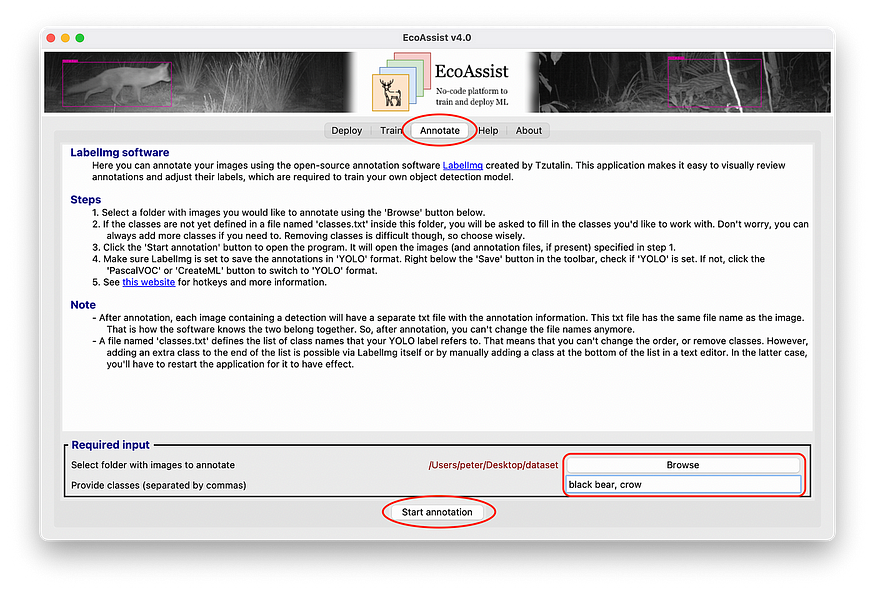
1.2 — Open EcoAssist and navigate to the ‘Annotate’ tab.
1.3 — Select the folder containing your images using the ‘Browse’ option.
1.4 — List the names of the classes you are interested in, separated by commas. For example: black bear, crow.
1.5 — Click the ‘Start annotation’ button. This will create a file called ‘classes.txt’ and open a new window in which you can label your images.
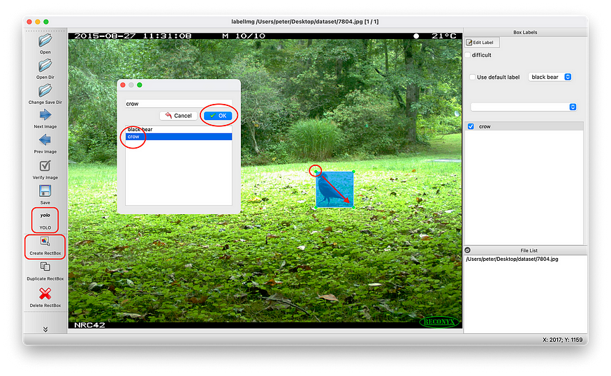
1.6 — Make sure the button just under the ‘Save’ button in the toolbar is set to ‘YOLO’. If you see ‘PascalVOC’ or ‘CreateML’, switch to ‘YOLO’.
1.7 — Click the ‘Create RectBox’ to draw a box around the object of interest and select the correct label. If all objects in the image are labeled, click ‘Save’ (or select ‘View’ > ‘Auto save mode’ from the menu bar) and ‘Next Image’. This will create a text file with the same filename as the image. Continue doing this until all objects in all images are labeled. When you’re done, the dataset should look like this:
─── U+1F4C1dataset
 U+007C──classes.txt
 U+007C──image_1.jpg
 U+007C──image_1.txt
 U+007C──image_2.jpg
 U+007C──image_2.txt
 U+007C──image_3.jpg
 U+007C──image_3.txt
 :
 U+007C──image_N.jpg
 └──image_N.txt
1.8 — Backup your final image dataset in case disaster strikes.
Step 2 — Train
In this phase, we’ll train a model to detect your objects.
2.1 — If you’re running this tutorial on a Windows computer, it might be useful to increase the paging size of your device before starting to train (FAQ 6, point 1). This will increase virtual memory and, thus the processing power of your device. This is not relevant for Mac and Linux users.
2.2 — Close all other apps to reduce background activities since training can place a significant demand on your machine.
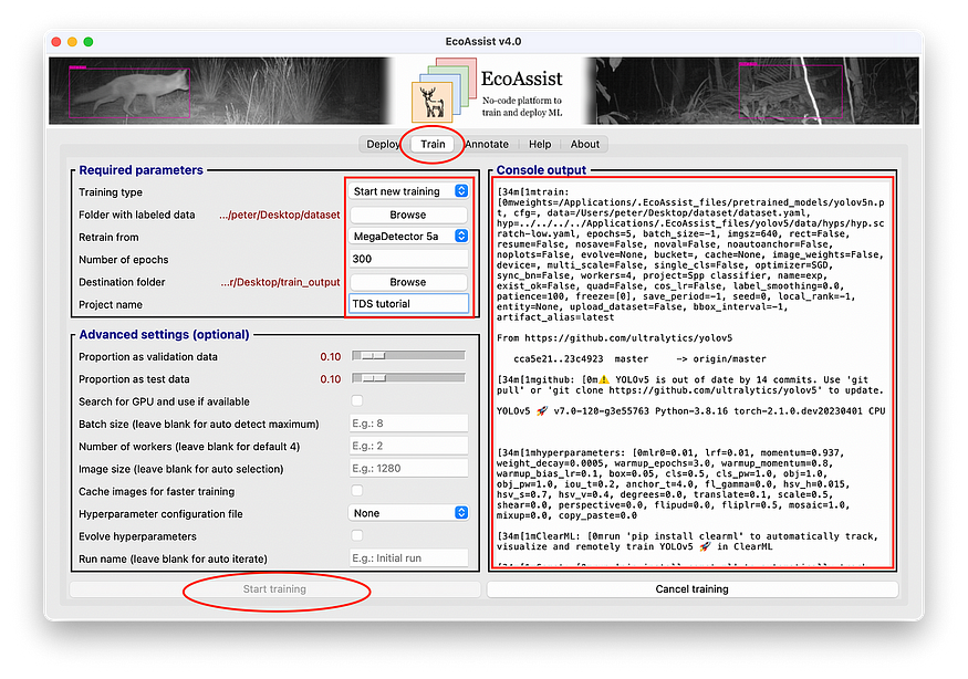
2.3 — Navigate to the ‘Train’ tab.
2.4 — Specify values for the required parameters.
- Training type — Here you can select whether you want to continue an existing training or start a new one. Leave it on the default ‘Start new training’.
- Folder with labeled data — Select the folder with images and labels created at the annotation step.
- Retrain from — Here, you can select which model you’d like to use for transfer learning. You can also choose to train your model from scratch. See FAQ 3 and FAQ 4 for more information about what is best for your project. If you’re training on the dataset of this tutorial, we’ll choose ‘MegaDetector 5a’.
- A number of epochs — An epoch means that all training data will pass through the algorithm once. This number thus defines how many times your computer will go through all the images. If this is the first time training on the data — go with 300 epochs.
- Destination folder — Select a folder in which you want the results to be saved. This can be any folder.
- Project name — This option will only appear after the destination folder is selected. Here you can choose a name for your project, e.g., ‘tutorial’. The project name option will be a dropdown menu if you selected a destination folder in which previous projects have already been stored.
2.5 — It’s possible to set values for more parameters, but it’s not mandatory. For this tutorial we’ll keep it simple. If you want to further fine-tune your training, take a look at the ‘Advanced settings’ and the ‘Help’ tab.
2.6 — Click ‘Start training’ to initiate the training process. You’ll see quite some output in the ‘Console output’ — most of which you can ignore. The training has begun if you see something like the output below. If you don’t see this, take a look at FAQ 5 and FAQ 6 to check whether you run out of memory and need to adjust the default settings.
Plotting labels to tutorial\exp\labels.jpg...
Image sizes 1280 train, 1280 val
Using 4 dataloader workers
Logging results to [1mincl-backgrounds\exp[0m
Starting training for 300 epochs...
 Epoch GPU_mem box_loss obj_loss cls_loss Instances Size
 0%U+007C U+007C 0/156 [00:00<?, ?it/s]
 0/299 10.6G 0.1024 0.06691 0.02732 20 1280: 0%U+007C U+007C 0/156 [00:03<?, ?it/s]
 0/299 10.6G 0.1024 0.06691 0.02732 20 1280: 1%U+007C U+007C 1/156 [00:08<21:48, 8.44s/it]
 0/299 10.6G 0.1033 0.06553 0.02709 15 1280: 1%U+007C U+007C 1/156 [00:09<21:48, 8.44s/it]
 0/299 10.6G 0.1033 0.06553 0.02709 15 1280: 1%U+007C1 U+007C 2/156 [00:09<11:01, 4.29s/it]
 0/299 11.5G 0.1035 0.0647 0.02714 14 1280: 1%U+007C1 U+007C 2/156 [00:11<11:01, 4.29s/it]
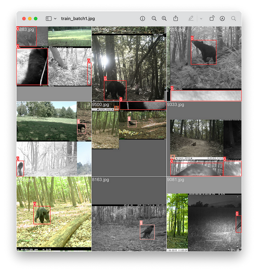
2.7 — If the training has begun, take a look at the train_batch*.jpg files in your destination folder. This is how your computer sees the data while training. It should correctly display the bounding boxes. An example is shown below.
2.8 — It’s possible to calculate how long the total process will approximately take when the training is running. If you see [02:08<01:09, 1.29s/it], it means that it’ll take an epoch (02:08 + 01:09 =) 3:17 min to complete. Multiply this with the number of epochs and you’ll have an estimation of the total time required for the training. Allow some extra time for data loading and testing after each epoch. However, please note that it might finish sooner than you think because it will automatically stop training if there hasn’t been any improvement observed in last 100 epochs.
2.9 — When the training is done, you’ll find the results in the destination folder you specified in step 2.4. We’ll evaluate these results in the next step.
Step 3 — Evaluate
When training an object detection model, it is very important to have a good understanding of your dataset and catch your final model while it has a good fit — meaning neither under nor overfit (FAQ 7). Therefore, we want to establish the point where the model starts to go from underfit to overfit, and stop training there.
3. 1 — Navigate to your destination folder and open results.png. See FAQ 8 for an elaborate interpretation of the metrics used in this graph and the rest of the files in your destination folder.

3.2 — The graphs above show the results of the data I’ve annotated for you. As you can see, it did not reach the set 300 epochs because of the built-in early stopping mechanism mentioned in step 2.8.
3.3 — See FAQ 7 to determine the point where your model has the best fit. In the example above, the model starts to get overfit around epoch number 50. If you’re doing this tutorial with your own data, it’s important to have actually overfitted the training in order to get a good understanding of your dataset and see the transition from underfit to overfit. If your data is not yet overfitted at 300 epochs, start a new training and select more epochs, e.g., 600 or 1200.
3.4 — Normally, the next step in the process would be to experiment with alternatives and optimize metrics (FAQ 9 and FAQ 10). However, for the sake of simplicity, we’re not going to optimize our model in this tutorial — we’ll accept the results as they are.
3.5 — Now that we’ve determined the point where our model has the best fit, we’ll need to stop the training there. We’ll do that by starting a new training with the same parameters as before but adjusting the number of epochs to the number with the best fit — in our case 50.
3.6 — When the training is done, open results.png again and inspect the results. You can choose to run another training if the new results.png provide better insight. After 50 epochs, my model has a precision of 0.98, a recall of 0.99, a mAP_0.5 of 0.99, and a mAP_0.5:0.95 of 0.77 — which is really good.
3.7 — You can find your final model in the destination folder: weights/best.pt. This is the actual model which can locate objects. You can move and rename it as desired.
Step 4 — Deploy
Your model is now ready for deployment.

4.1 — Navigate to the ‘Deploy’ tab.
4.2 — Select a folder with images or videos you’d like to analyze at ‘Browse’. If you don’t have any test images, you can download some from my Google Drive (≈5MB).
4.3 — Select “Custom model” from the dropdown menu at the ‘Model’ option and select your model created at the previous step.
4.4 — Tick the checkboxes to analyze images and/or videos.
4.5 — Select any other options you’d like to enable. See the ‘Help’ tab for more information about those.
4.6 — Click ‘Deploy model’.
Step 5 — Post-process
At this point, you have successfully trained and deployed your own object detection model. All the information you need is in the image_recognition_file.json for images or video_recognition_file.json for videos. You can use this file to process the images to your specific needs in Python, R or another programming language of your choice. However, I understand that programming can be a bit daunting, and I have thus prepared some generic post-processing features which will hopefully help you on your way.
- Separate files into subdirectories — This function divides the files into subdirectories based on their detections. For example, they will be divided in folders called
black bear,crow,black-bear_crow, andempty. - Draw bounding boxes and confidences — This functionality draws boxes around the detections and prints their confidence values. This can be useful to visually check the results.
- Crop detections — This feature will crop the detections and save them as separate images.
- Create annotations in YOLO format — This function will generate annotations based on the detections. This can be helpful when generating new training data. You’ll just have to review the images and add them to your training data.
- Export results in csv files — This will transform the JSON files to CSV files to enable further processing in spreadsheet applications such as Excel.
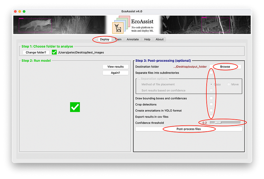
Follow the steps below to execute these post-processing features. The ‘Post-processing’ frame will become available after the deployment has finished.
5.1 — Select the folder in which you want the results to be placed at ‘Destination folder’.
5.2 — Tick the checkbox of the post-process feature you’d like to execute. It’s possible to select multiple.
5.3 — Select a confidence threshold to determine the minimum confidence. Detections below this value will not be post-processed to avoid false positives. If you don’t know what the best value is, read the explanation in the ‘Help’ tab or just stick with the default value.
5.4 — Click ‘Post-process files’.
As you can see, the model correctly located all the bears and crows, whilst ignoring all the other animals and backgrounds. Job well done! Now it’s time to test it on a bigger scale…

Conclusion
I hope I’ve demonstrated a simple method of working with object detection models and you’ll now be able to use AI in your projects. Try to expand your dataset by collecting new images and improve model metrics by training a new model on this growing dataset every now and again. Once you have a working model, export YOLO annotations together with your new images so you don’t have to label everything manually. You’ll just have to review and adjust them before they’re ready for training.
Since EcoAssist is an open-source project, feel free to contribute on GitHub and submit fixes, improvements or add new features.
Frequently asked questions
- What kind of computer should I use for object detection?
- What should a good training dataset look like?
- How to choose between transfer learning or training from scratch?
- Which model should I choose when transfer learning?
- How does it look when I run out of memory?
- What should I do when I run out of memory?
- How can I recognize overfitting and when does my model have the best fit?
- What are all the files in the training folder and how should I interpret them?
- What’s the general workflow of an object detection training?
- What can I do to avoid overfitting and optimize my model?
References
- van Lunteren, P. (2022). EcoAssist: A no-code platform to train and deploy YOLOv5 object detection models [Computer software]. https://doi.org/10.5281/zenodo.7223363
- S. Beery, D. Morris and S. Yang, Efficient pipeline for camera trap image review (2019), arXiv preprint arXiv:1907.06772.
- H. Yousif, R. Kays, H. Zhihai, Dynamic Programming Selection of Object Proposals for Sequence-Level Animal Species Classification in the Wild (2019), Institute of Electrical and Electronics Engineers: Transactions on Circuits and Systems for Video Technology.
Join thousands of data leaders on the AI newsletter. Join over 80,000 subscribers and keep up to date with the latest developments in AI. From research to projects and ideas. If you are building an AI startup, an AI-related product, or a service, we invite you to consider becoming a sponsor.
Published via Towards AI
Related posts


Popular posts

 for 2021")


Updates

Recent Posts


