Boost Your Job Search With NLP

Author(s): Gabriele Albini

Originally published on Towards AI.

Presenting a web app with semantic search functionalities based on pre-trained sBERT, and a Plotly Dash interface U+007C Live app U+007C Git Hub

Introduction

In the most common job platforms, search functionalities consist of filtering jobs based on a few input words plus some filters (such as location). These words generally indicate a domain or a desired position, and, in most cases, the exact input words “must” appear in the job descriptions that the search system retrieves. We’re not exactly sure to what extent the latest NLP (Natural Language Processing) techniques are used to optimize our search.

NLP has recorded remarkable breakthroughs in recent years, and we can leverage some techniques that are able to bring search to the next level. We can think of using semantic search based on a set of query-sentences indicating, e.g.:

• the tasks we would like to perform in the next job
• the ideal working context, such as the company culture
• (for tech jobs) the tech stack we wish to use

In this article, we will recap how sBERT (sentence BERT) model works and will show how to apply a pre-trained model to improve daily tasks like searching for a job.

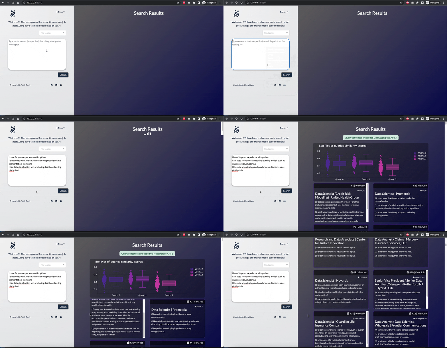
A Dash app has been built, including these search functionalities; here’s what it looks like:

Table of Content

1. What is sBERT?
1.1 Quick review of NLP embeddings techniques
1.2 Transformers overview
1.3 From transformers to sBERT
1.4 From BERT to sBERT
2. Generating sentence embeddings
2.1 Choosing among pre-trained models
2.2 Using pre-trained models for semantic search
3. Putting all together with Dash
3.1 Data preparation
3.2 App Input
3.3 Matching mechanism
References

1. What is sBERT?

1.1 Quick review of NLP embeddings techniques

For any NLP tasks (like search) we need to represent our text into vectors, such that we can perform mathematical operations. There is now a vast history of embeddings techniques:

• “Bag of words”: these traditional methods use word frequencies in documents or terms co-occurrences to create embeddings at the word (or document) level. Each vector consists of binary entries or frequency entries (there are several ways of measuring frequencies: tf-idf, ppmi, bm25, …). The resulting vectors are often too big and sparse.
• “Count-based models”: these models overcome the limitations of size/sparsity vectors of the above approaches. Starting from term co-occurrences matrices (or document-term matrices), dimensionality reduction techniques are applied to create dense and smaller vectors. Some examples of these approaches are GloVe (which uses an enhanced version of SVD, singular-value decomposition, to reduce size), LSA (latent semantic analysis).
• “Predictive models”: these models use simple (1 hidden layer) neural networks trained to predict a word. Word2Vec is a very famous model (more details here) that can be trained to predict a target word starting from some surrounding words (using a fixed window) or vice-versa (predicting the context from a given word). The weights learned by the hidden layer can be used as word embeddings.
• “Contextual embeddings”: the more recent research focused on creating word representations that take context into account. In fact, models like Word2Vec create a “global” representation of each word and there are some obvious limitations (think of polysemy, context-dependent terms, …). Contextual embedding models can create dynamic word representations that change depending on the context, word type (noun/verb), grammar rules, etc. These models are based on deep neural networks. For some time, different types of RNN (recurrent neural networks) (LSTM, GRU) were proposed, with some limitations: (a) these architectures were computationally slow as they need to be trained sequentially; (b) they presented some limitations when relating words that are very far in the corpus. All these limitations were overcome by Transformers, a network architecture created by Google [1], that inspired the creation of many different models, such as BERT, GPT, etc.

1.2 Transformers overview

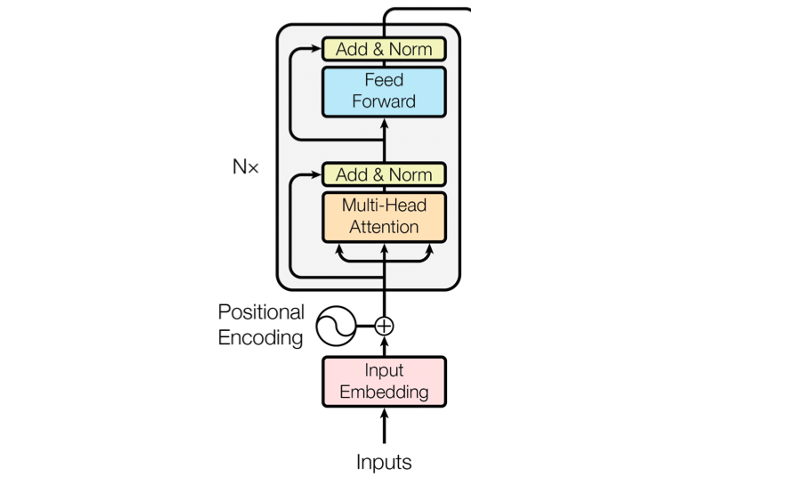
Transformer neural networks were presented on machine translation tasks. They have an encoder architecture and a decoder architecture. Since in this post, we are interested in using Transformers for text embedding, we will be only focusing on the encoder part:

• Input Embedding: transformer architecture takes as input, for each word, an embedding vector of dimension 512 (the input embedding is an initialization that will be later improved).
• Positional encoding: since transformers take as input all the word embeddings at the same time (and not word by word like RNN), they need some extra information about the position of each word. This is why the input embedding vectors are summed to positional vectors. Each positional vector is built using Fourier series theory: the sin and cos functions are used to get a unique vector depending on the position of the word in the sentence (pos) and on the i-th dimension of the vector (i). For each word and dimension, the positional score is added to the corresponding embedding. (Watch this for a graphical and more exhaustive explanation).
• Self-attention mechanism: Intuitively, an attention mechanism allows the model to assign more weight to those parts of the input which are relevant to complete a task. There are clear examples of this mechanism in computer vision (e.g., object detection), where CNNs (Convolutional Neural Networks) learn “filters” to be applied to an image so that the network can focus on the relevant pixels. This concept was applied to NLP as well, using Q (query), K (keys), V (values) matrices. These matrices are initially just copies of the input vectors. The Q, and K matrices are multiplied to build a “mask” matrix, i.e., a matrix containing attention scores for each pair of terms. Thanks to the multiplication, similar pairs will get higher scores (the softmax function constrains these scores from 0 to 1). This attention filter is then multiplied by the V matrix, to get a weighted value for each pair of terms. Intuitively, this method allows to link each term to other parts of the input sentence to complete a task (e.g., machine translation) (watch this for a graphical and more exhaustive explanation):

• Multi-head attention: the above attention mechanism is repeated multiple times. Intuitively, this means that the model learns the tasks from different points of view: one layer may use attention with respect to vocabulary, another layer with respect to grammar, etc.

As an output of the whole encoding layer, we obtain a matrix with all embedding vectors. These vectors store the word embedding, the positional encoding information, and the context information (i.e., what other words in the sentence got prioritized by the attention layers).

1.3 From transformers to BERT

Since the Transformer paper, several models have been created using variations of this architecture for specific purposes.

BERT (Bidirectional Encoder Representations from Transformers) was created by Google in 2018 [2] using only the encoder component of the transformer architecture. The idea of this model was to create a versatile pre-trained model that could produce contextual semantic embeddings that could be passed into a fine-tuning step. In simple terms: a user, depending on a specific task, could use a pre-trained BERT model and add a fine-tuning layer to complete the training (e.g., depending on a specific classification task).

Compared to the original encoder, the BERT model:

• Adds some modifications to the architecture: it stacks a bigger number of transformer encoders (12 in the “BERT base” version and 24 in the “BERT large” version); it adds more multi heads in the self-attention mechanism (12 in the “BERT base” version and 16 in the “BERT large” version); the final embedding vectors have bigger sizes (768 in “BERT base” and 1024 in “BERT large”).
• BERT is trained on two unsupervised tasks described below.

The two tasks are:

• Masked LM (MLM): predict a word that was corrupted in the input. Practically, during training, 15% of the tokens from the input sentences were “masked” in three different ways (80% of the time, the token was replaced by a [MASK] token; 10% by a random word; 10% left unchanged). The encoder was trained to predict these tokens.
• Next sentence prediction (NSP): BERT was trained to learn the relationship between two sentences to improve question-answering or inference performances. When a pair of sentences A, B were given as input (separated by a special [SEP] token), 50% of the time, B was the natural sentence that followed A, while 50% of the time, B was a random sentence. The encoder was trained on predicting the “isNext” label relating A to B.

1.4 From BERT to sBERT

A sBERT (sentence-BERT) model was created in 2019 [3] to improve the BERT model for specific tasks such as sentence similarity or sentence clustering. The sBERT paper highlighted the following “weak” points in the original BERT model:

• BERT was trained on NSP, but that is not exactly predicting how similar the two sentences A, and B are.
• BERT requires two input sentences in order to compare them, this would slow down the computation when looking for the most similar sentences in a corpus.
• BERT doesn’t output a single sentence embedding. (Several strategies were tested to extract a sentence embedding from BERT, but a unanimous method wasn’t found).

The sBERT model was created with the following architecture:

• A BERT model is used to produce an embedding for each sentence. As discussed, since there’s not a single way to extract sentence embeddings from BERT, the sBERT default way is to calculate a mean on all the transformer outputs. Then, a “pooling” layer is added to calculate fixed-size sentence embeddings (independently from the sentence length).
• sBERT uses Siamese networks (two copies of the same architecture), trained on different tasks (e.g., sentence classification and regression — the picture refers to this second case, i.e., predicting the sentence similarity). Depending on the task, the objective function at the top level of the architecture can be modified.

Thanks to pre-trained sBERT models, we can create sophisticated sentence embeddings of fixed sizes in a computationally efficient way! Let’s see an example below.

2. Generating sentence embeddings

2.1 Choosing among pre-trained models

Since the sBERT release, many pre-trained models were built and compared on several tasks.

To pick a model, first of all, let’s focus on the ones designed for our task. In this post, we want to find a model for semantic search, which can be of two types:

• Symmetric search: we have a symmetric search when the query and the result are approximately of the same size and of similar content.
• Asymmetric search: we have an asymmetric search when the query is short, and the expected result is a longer sentence answering the query.

We’ll be performing a symmetric semantic search: here’s a list of the top-performing models pre-trained on this task. At the time of the article, the top-performing model is all-mpnet-base-v2 [4], which:

• is pre-trained on predicting sentence similarity using above 1 billion sentences
• allows input sentences of max 384 tokens words (longer input is automatically truncated)
• outputs embeddings of size 768

2.2 Using pre-trained Models for semantic search

Let’s see the above model in action.

Suppose we have extracted these two sentences from two job descriptions. One is looking for candidates with churn models experience, the other is looking for candidates with nlp experience:

A user, who is looking for jobs aligned with his/her experience in customer analytics, types the following query:

Note how there’s no word overlapping between the query and the two sentences. Traditional models would fail to relate the query to one of the two sentences unless encoding some semantics and contextual information.

Let’s download the sBERT model from Huggingface and encode all three sentences:

Alternatively, we can also use Huggingface API to request embeddings:

We can now calculate the cosine similarity between the query and each job sentence:

And then plot the embeddings (we’ll use tSNE to reduce the embeddings to 3 dimensions):

We can see how “job 0” was successfully selected as more similar to the query. The model “knows” that churn models are more related to customer satisfaction and retention, compared to nlp !!!

3. Putting all together with Dash

We can now build a Dash web application that simulates a search system. This app has been deployed using Python anywhere, here.

3.1 Data preparation

Before starting our search, we should prepare the data, clean it and produce embeddings for each sentence:

• We assume some job description data to be available. To get this data, we can scrape job platforms (here’s one example).
• The data needs to be pre-processed, using classic NLP techniques, and tokenized into sentences (here’s the code used for this project).
• In the app I have designed, two dataframes are used. One (“Job_Info”) contains all job information (such as: job ID, location, employer, full description) and the other (“df_embeddings”) contains sentences, one per row.
• Using the sentence dataframe, we produce sentence embeddings using a copy of the pre-trained sBERT model (The sentence embeddings are saved directly into “df_embeddings”).

3.2 App Input

The app requires user input to work. The user will need to:

• Write some query sentences. The app manages up to 10 query sentences.
• (Optional) Select among the available locations.

Once the “Search” button is pressed, the app will use the Huggingface API to embed each query sentence (the model and code used are shown above). (If you want to set up a copy of this app locally, remember to input your own API token in “.assets/nlp_functions.py/embed_api”).

Here’s how the input interface looks like:

3.3 Matching mechanism

To rank jobs, the app computes the cosine similarity of each job sentence against each query sentence.

The maximum similarity for each job and query sentence will be saved. So, supposing we have 4 input query sentences, each job will have 4 similarity scores.

Using these similarity scores, each job is ranked from 1 (top similarity) to n.

Finally, the different ranks are combined using a weighted average to generate a single final ranking score per job. Here’s why and how:

• Suppose we have two input query sentences. Across all job sentences, query-1 has a max of 0.2 similarity, while query-2 has a max of 0.8.
• If we pick a job (comparing cos similarities from all its sentences) that ranked 1st on query-1 but 10th on query-2, we may want to prioritize other jobs that scored worse in query-1 but better in query-2.
• So, a weighted average of individual job ranks is computed using the max similarities obtained in each query.

Finally, the app produces two outputs:

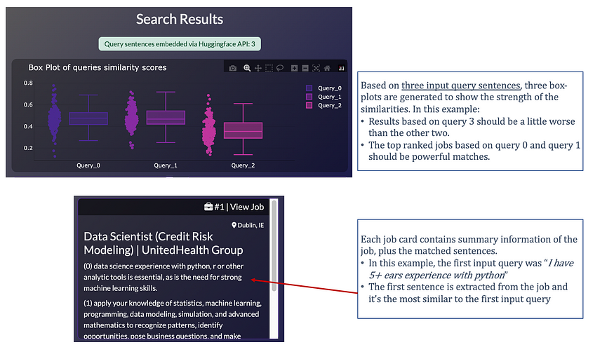
• A box-plot showing the “strengths” of similarity scores between jobs and query sentences. One box plot is generated per query sentence, where individual data points are the max similarity scores of each job. With this chart, we can immediately see if our query sentence produced “strong” matches.
• Ranked results: one dbc.Card is generated per job, from most similar to least similar jobs. Each job card contains the sentences, extracted from the full job description, used by the system to rank the job.

Here’s how the output interface looks like:

I hope this was useful and that you may apply this in your own job search. Thank you for reading!!!

References

• [1] “Attention is all you need” (2017) — Vaswani, Noam Shazeer, Niki Parmar, Jakob Uszkoreit, Llion Jones, Aidan N Gomez, Lukasz Kaiser, and Illia Polosukhin. Annotated version with implementation notes, code reviews, and examples.
• [2] “BERT: Pre-training of Deep Bidirectional Transformers for Language Understanding” (2018) — Jacob Devlin, Ming-Wei Chang, Kenton Lee, and Kristina Toutanova
• [3] “Sentence-BERT: Sentence Embeddings using Siamese BERT-Networks” (2019) — Nils Reimers, and Iryna Gurevych
• [4] Huggingface “all-mpnet-base-v2” model

Join thousands of data leaders on the AI newsletter. Join over 80,000 subscribers and keep up to date with the latest developments in AI. From research to projects and ideas. If you are building an AI startup, an AI-related product, or a service, we invite you to consider becoming a sponsor.

Published via Towards AI