The Multilayer Perceptron: Built and Implemented from Scratch

Author(s): David Cullen

 

Originally published on Towards AI.

This article aims to provide an overview of the multilayer perceptron, covering key areas mathematically, visually, and programmatically.

An approach has been adopted to enable the reader to capture the intuition behind a multilayer perceptron using a bite-size, step-by-step method.

Background reading relating to matrix multiplication, linear algebra (linear transformation), algebraic expression simplification, and calculus (derivatives, partial derivatives, and chain rule) will support the reader in getting the most out of this article. Additionally, experience with Python will aid the reader in understanding the application of the multilayer perceptron architecture discussed in this article.

Key concepts include: binary classification, neural network forward propagation, backpropagation, binary cross-entropy loss, and gradient descent.

Model Architecture:

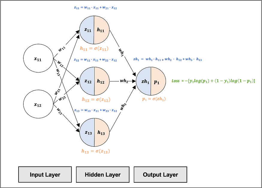
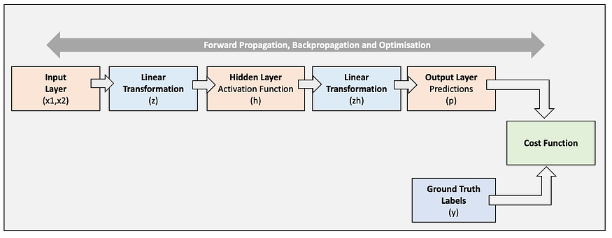
We will create a multilayer perceptron (MLP), which is a feedforward neural network. In this model, inputs are multiplied by weights, summed, and passed through a non-linear activation function that activates each input. The activated data from the hidden layer is then sent to the output layer that provides the prediction. An overview of the model architecture has been provided below:

Input Layer: we will use 2 inputs (x1 and x2), relating to each feature in each training example.

Hidden Layer: we will include a layer in between the Input Layer and Output Layer, consisting of 3 neurons (h1,h2, and h3).

Output Layer: we will use a layer for the prediction (p) consisting of one neuron.

Fig 1. visualizes the MLP Architecture we will implement.

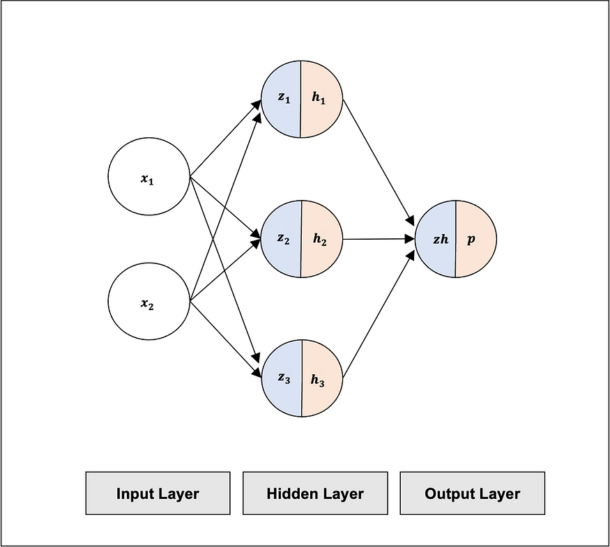
x : input feature at input layer

z : linear transformation to the hidden layer

h: activation function at the hidden layer

zh: linear transformation to the hidden layer

p : prediction at the output layer

Training Examples:

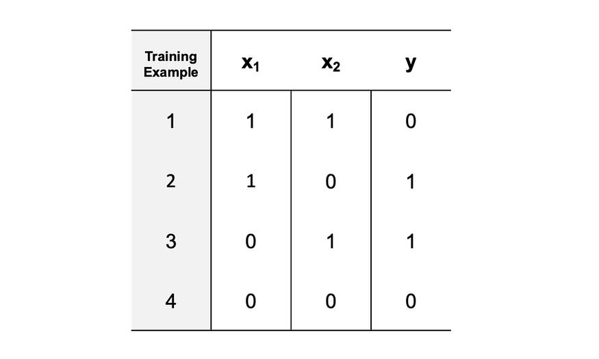
We will want to train our MLP neural network so it can learn patterns in the data. For the purposes of simplicity, we will use XOR logic gates to train the data. An XOR logic gate produces a true output (y = 1) if the number of true inputs is odd.

Table 1 provides an overview of the XOR logic gate data we will use to train the network.

As shown below, the number of training examples is 4. For each training example, two input features (x1 and x2) will be used. Each training example has a corresponding y output. The y output is the ground truth label that will be compared to the MLP output prediction (p) to assess the performance of the model.

Important Note: This article focuses on training an MLP. Following training, MLPs are evaluated on unseen data, referred to as test data. This assesses how well the MLP generalises. The evaluation of the MLP on test data is outside the scope of this article.

Building the Multilayer Perceptron

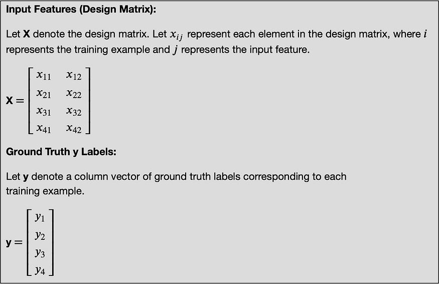
Step 1: Input Features (Design Matrix) and Ground Truth y Labels

We will first store the input features (x1, x2) for each of the 4 training examples in a matrix known as the design matrix. We will also store the corresponding ground truth y labels in a column vector.

Fig. 2 provides an overview of the design matrix and y-label column vector.

Step 2: Forward Propagation

Now that we have defined the model and training data, we can forward feed the inputs to arrive at the output. In order for this, we will need to do the following:

Model Parameters: initialise the model’s weight coefficients (w and wh) and perform a linear transformation on each input to the hidden layer and the output layer.

Note: For simplicity we will not include the bias in the linear transformations used in this article. The bias (b) is the additive constant in linear functions wx+b, used to offset the result and shift the activation function.

Activation Function: define the non-linear activation function and pass parameterised inputs to it.

Loss/Cost Function: define the loss/cost function that we will use for assessing the difference between the ground truth labels and the associated model predictions.

Further detail has been provided below:

Model Parameters :

The weight coefficients are the parameters of the network. We will initialize them from a random Gaussian distribution, which has a mean of 0 and a variance of 1. By doing this, there will be a higher chance to draw weights close to the mean, resulting in more stable weight values used to initialize the network. These weights will later be updated by the network to optimize its prediction ability (more on this below).

The total number of parameters (weights) used in this network is 9. This can be worked out by multiplying the number of neurons at the Input Layer by the number of neurons at the Hidden Layer (2 x 3 = 6) and the number of neurons at the Hidden Layer by the number of neurons at the Output Layer (3 x 1 = 3).

Weight Matrix (Input to Hidden Layer): As we have 4 training examples, we will first create a weight matrix to store the weight coefficients from the Input Layer to the Hidden Layer (6 weights).

Fig. 3 provides an overview of the weight matrix.

Note: For additional context, please refer to Fig 6, where the connections of each weight coefficient connecting to the Hidden Layer can be identified.

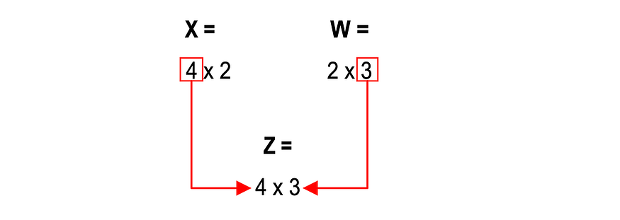
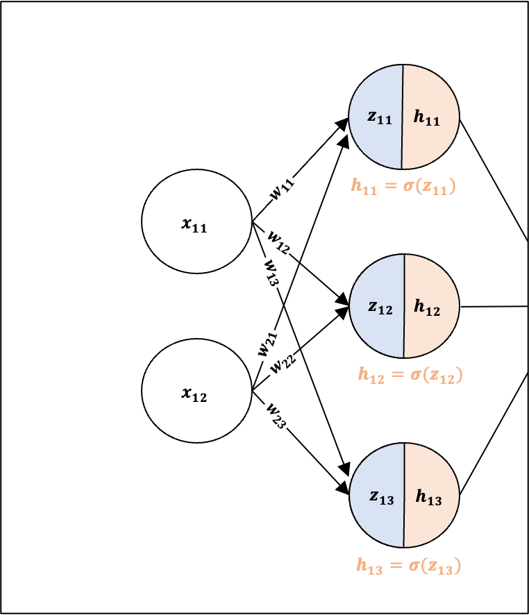
Linear Transformation (to the Hidden Layer): We will perform a linear transformation on each input (x) feature passed to the Hidden Layer. This means the model can learn linear relationships in the data. To do this, we will perform matrix multiplication on each input feature and associated weight coefficient. The design matrix has dimensions of 4 x 2, and the weight matrix is 2 x 3 (as shown above). Multiplication of these two matrices results in a new 4 x 3 Z matrix, where each row represents each of the 4 training examples and each column represents a z node. This has been illustrated in Fig. 4 and Fig. 5:

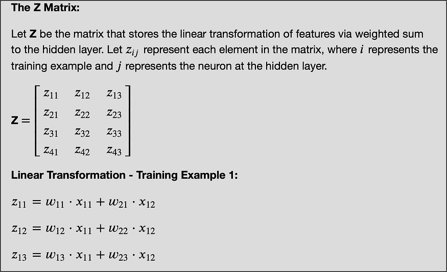
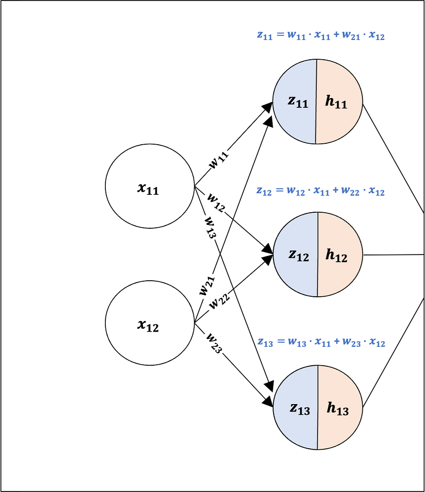
The linear transformation for training example 1 has been visualized in Fig 6, demonstrating the linear transformation of the two input features via weighted sum at each z node.

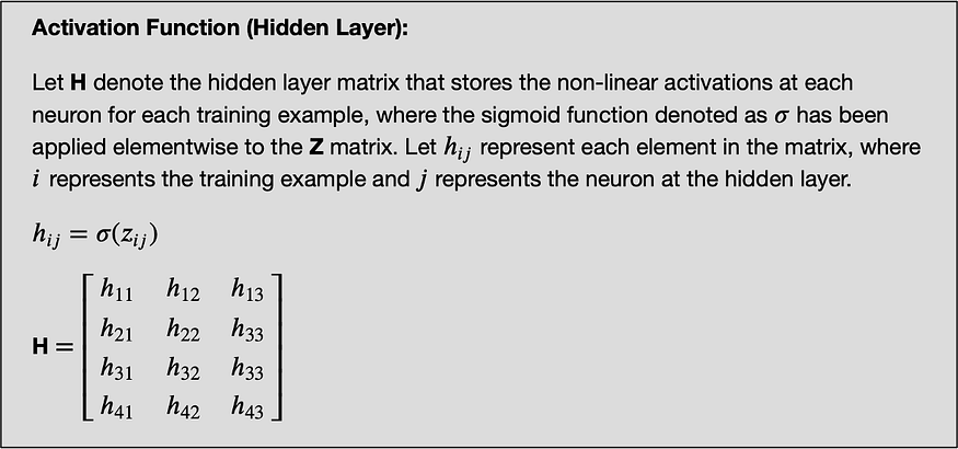
Activation Function (Sigmoid Function):

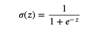
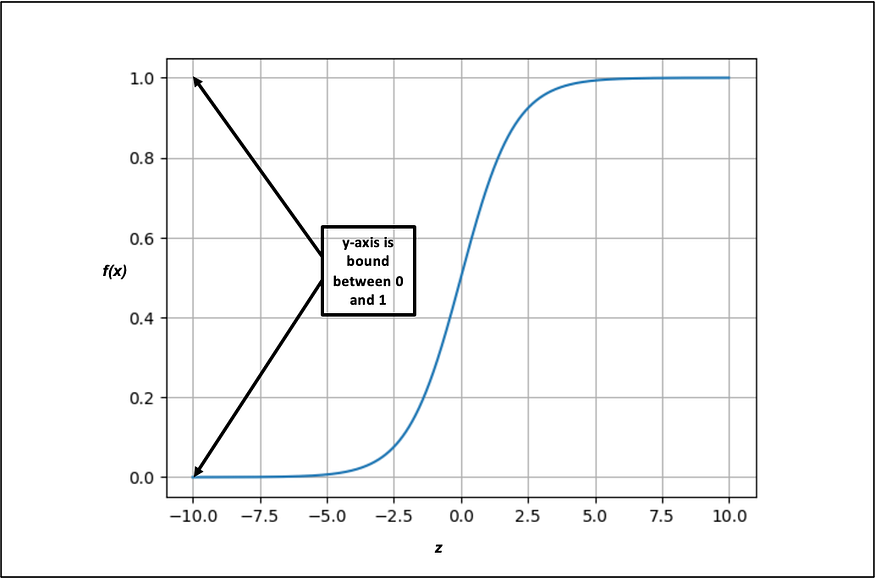
Our next step is to include a non-linear activation function that will adjust the level of activation of each neuron at the Hidden Layer and Output Layer. For this, we will use the sigmoid function. It takes a value (z) and squashes it between 0 and 1. For instance, if we pass the value -10 to the sigmoid function, it will return a value close to zero. The closer to 0, the less activated the neuron is, and the closer to 1, the more activated it is. The idea is that the more positive the neuron is, the more active it is, inspired by the human brain — taking us beyond linearity!

The mathematical representation and visual intuition of the sigmoid function have been provided below:

Activation Function (at the Hidden Layer): Now that we have defined the activation function, we can use it at the Hidden Layer. In order to do this, we apply the sigmoid function to each element in the Z matrix for each training example, as detailed in Fig.9 :

The activation function at the Hidden Layer for training example 1 has been visualized in Fig.10:

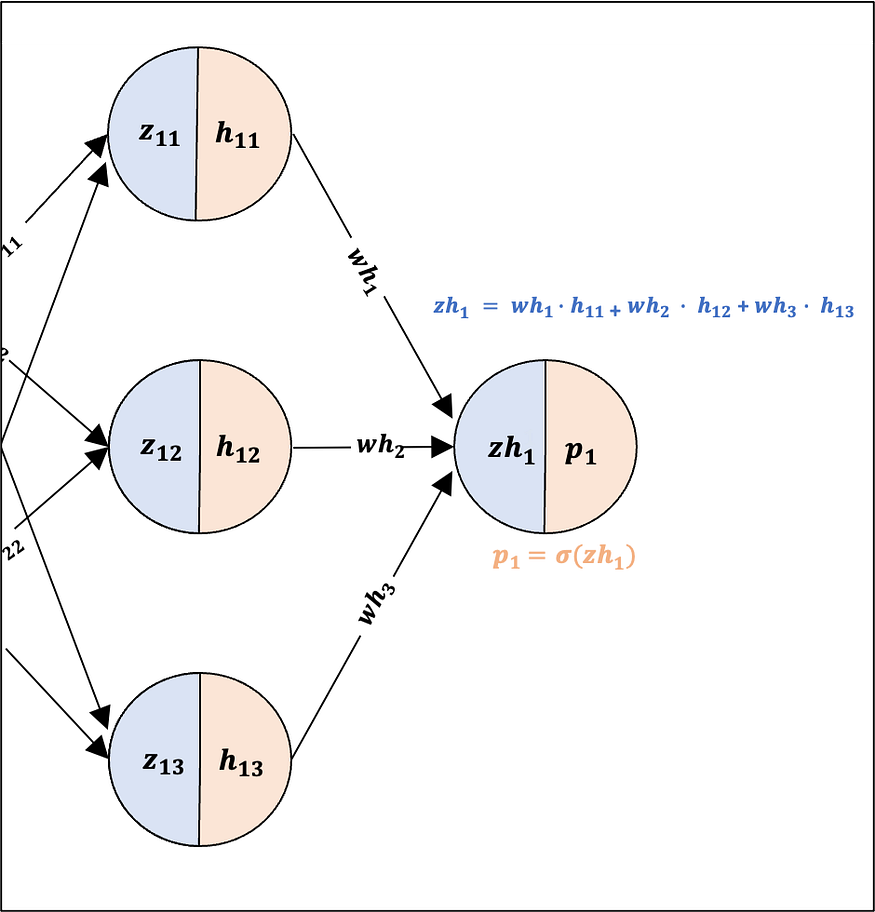
Output Layer Prediction: We will now perform a linear transformation and apply the sigmoid function from the Hidden Layer to the Output Layer, resulting in the predicted output (see Fig. 11 below). By using the sigmoid function, the predictions of our model are bound between 0 and 1. These bound values can be viewed as the predicted probabilities of the model.

The linear transformation and prediction at the Output Layer for training example 1 has been visualised below:

Loss and Cost Function: Binary Cross Entropy Loss/Cost Function

The Loss and Cost functions show us the difference between the ground truth y labels and the associated predictions. In particular, the Loss function shows the difference for one training example, whereas the Cost function shows the average difference across all training examples.

We will use the Loss function for the purposes of explanation and intuition below:

Binary Cross Entropy Loss: If you recall, the predictions of our model are bound between 0 and 1. Using the Binary Cross Entropy Loss, we can compare each of the model’s predictions to the associated ground truth (y) labels.

The Binary Cross Entropy Loss has been mathematically represented in Fig. 13.

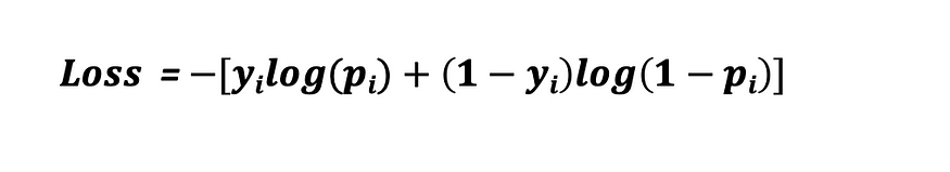
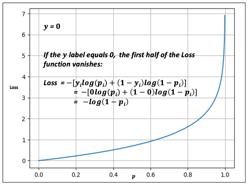
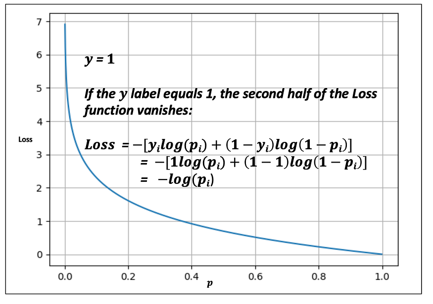
Using the negative log, the Binary Cross Entropy Loss heavily penalizes incorrect predictions the further they are away from the ground truth y label. This has been intuitively illustrated in Fig. 14 and Fig. 15.

If y = 0, the closer p gets to 1 results in a rapidly increasing Loss. Alternatively, the closer p gets to 0, the closer the Loss is to 0.

If y = 1, the closer p gets to 0 results in a rapidly increasing Loss. Alternatively, the closer p gets to 1 the closer the Loss is to 0.

Binary Cross Entropy Cost Function: We can take the average Loss between the ground truth y labels and predictions over all training examples to optimize the overall model’s performance.

To assess the model’s overall performance, we will use the Binary Cross Entropy Cost Function, which has been mathematically described as follows:

Note: The natural logarithm has been used for both the Binary Cross Entropy Loss and Cost Function.

Forward Propagation (Input Layer to Output Layer Summary):

Fig 17. brings together the forward propagation we have covered above, from the Input Layer to the Output Layer, for one training example.

Step 3. Backpropagation:

Our model has produced a number of predictions, but they might not be the best predictions the model can achieve. We can attempt to optimize the model and improve its predictions by adjusting its weights a nudge. Before we do this, let’s cover a few related concepts at a high level:

Derivative: The derivative of a single variable function (such as f(x) = x² ) is the instantaneous rate of change at a given point of a function.

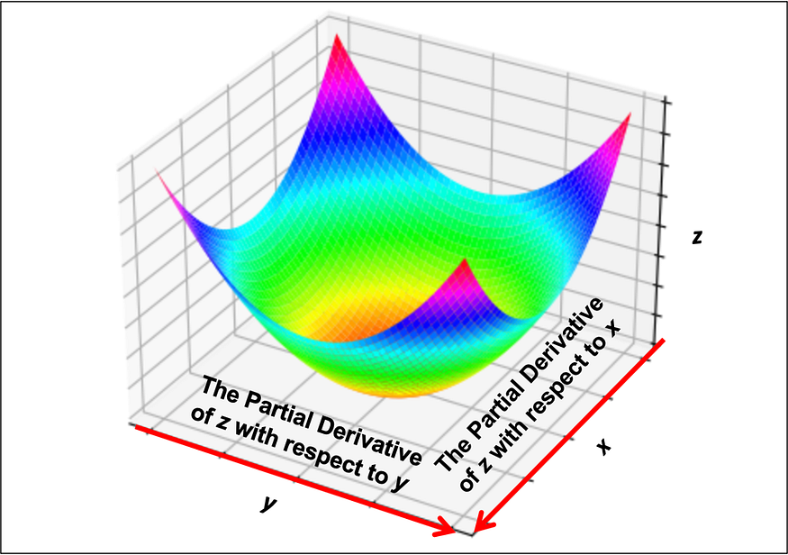
Partial Derivative: For multivariable functions such as z = x² + 2y² , we take the partial derivative of x, treating y as a constant (and vice versa for the partial derivative of y). ∂, also known as del, is used to indicate the partial derivative.

A visual has been provided below to demonstrate the partial derivative with respect to x and y, where z is a function of x and y.

Composite Functions & Chain Rule: Composite functions are functions within functions and can be written as follows: f(g(x)). As one can see there is an inner function g(x) and outer function f(x). A simple example of a composite function would be f(x) = sin(x²). In this example, f(x) = sin (x) is the outer function, and g(x) = x² the inner function.

The chain rule states that the derivative of a composite function, is equal to the derivative of the outer function evaluated at the inner function multiplied by the derivative of the inner function evaluated with respect to the variable of differentiation. This rule also applies to the partial derivative of a composite function.

MLP Backpropagation:

Our neural network can be described as a composition of multiple functions: p(zh(h(z(x)))), where x is the input at the Input Layer, z is the linear transformation of x, h is the sigmoid activation function at the Hidden Layer, zh is the linear transformation of h, and p is the sigmoid function prediction of the model at the Output Layer.

Our Binary Cross Entropy Loss function takes the neural network prediction (p) as an input, along with the ground truth label (y).

The partial derivative is particularly important for neural networks. This is because the partial derivative of the Loss function with respect to each weight is calculated and then nudged a small amount to improve the model’s predictions. Updating the weights in this manner means that we can aim to find the minimum of the Loss function, which in turn enables us to find the optimal prediction (more on this later).

In order to update the weights, we will perform backpropagation, using the chain rule to find the partial derivative of each weight with respect to the Loss.

Using the neural network we have built so far, we will demonstrate the partial derivative and chain rule in action for one training example and two weights (w11 and wh1):

The partial derivative of the Loss with respect to wh1:

We will want to nudge wh1 by a small amount to assess its impact on the Loss. To do this, we first need to find the partial derivative of the Loss with respect to wh1.

We cannot directly access the partial derivative of the Loss with respect to wh1. To overcome this, we need to move downstream using the chain rule, starting with the partial derivative of the Loss with respect to p1 (see Fig 20 and 21 for further details).

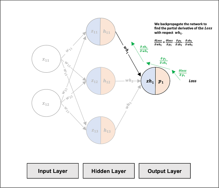
The following schematic demonstrates how the above partial derivatives relate to one another:

• ∂loss/∂p1 represents the sensitivity of the Loss function to changes in p1.
• ∂p1/∂zh1 represents the sensitivity of p1 function to changes in zh1.
• ∂zh1/∂wh1 represents the sensitivity of zh1 function to changes in wh1.

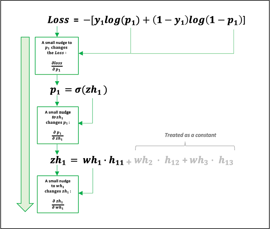
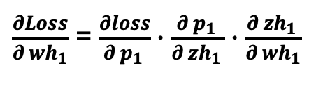
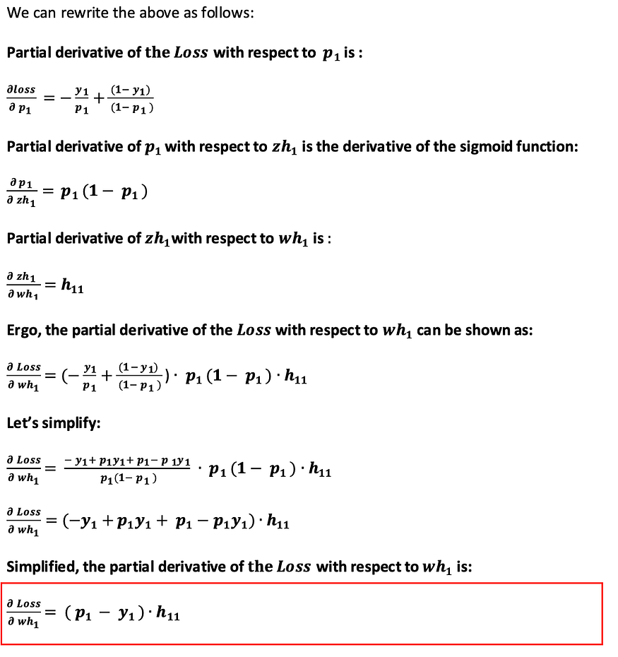
By taking the above partial derivatives and multiplying them together (using the chain rule), we can find the partial derivative of the Loss with respect to wh1:

The partial derivative of the Loss with respect to w11:

Next, we will want to nudge w11 by a small amount to assess its impact on the Loss. Similarly, we cannot directly access the partial derivative of the Loss with respect to w11. We, therefore, need to move downstream using the chain rule, starting with the partial derivative of the Loss with respect to p1 (see Fig 23 and 24 for further details).

Note: we can use the first two partial derivatives (∂loss/∂p1 and ∂p1/∂zh1) already calculated as part of ∂loss/∂wh1 above (see fig 22). Hence the efficiency of backpropagation!

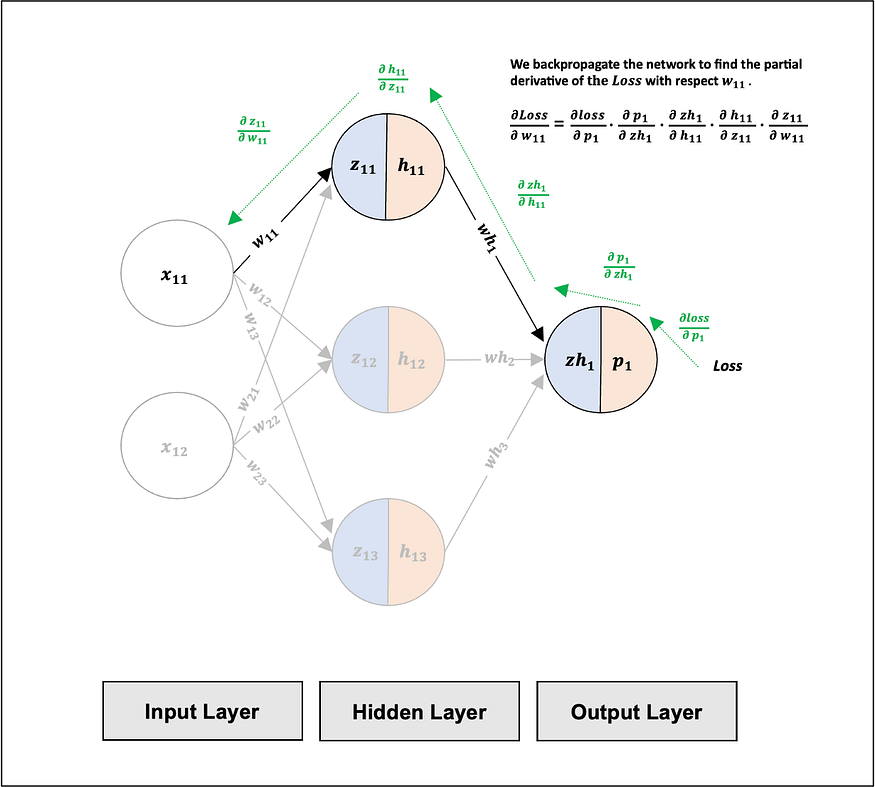
The following schematic demonstrates how the above partial derivatives relate to one another:

• ∂loss/∂p1 represents the sensitivity of the Loss function to changes in p1.
• ∂p1/∂zh1 represents the sensitivity of p1 function to changes in zh1.
• ∂zh1/∂h11 represents the sensitivity of zh1 function to changes in h11.
• ∂h11/∂z11 represents the sensitivity of h11 function to changes in z11.
• ∂z11/∂w11 represents the sensitivity of z11 function to changes in w11.

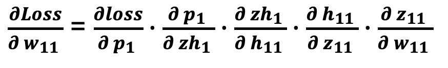
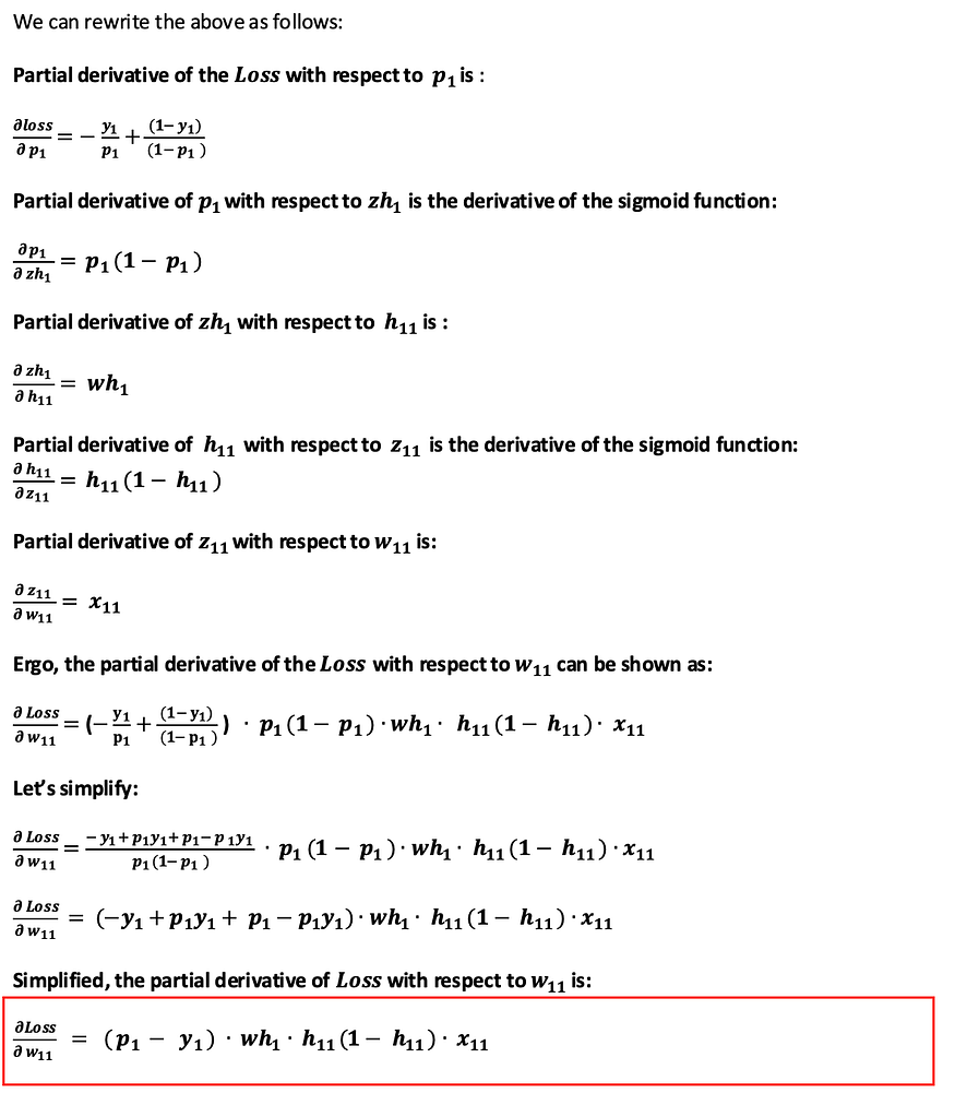
The partial derivative of the Loss with respect to w11 can be represented as:

The partial derivative of the Loss with respect to the model’s remaining weights will need to be calculated using the procedures mentioned above.

Optimization: Gradient Descent and Learning Rate

Now that we have calculated the partial derivatives for the Loss with respect to each weight, we can adjust these weights by a small amount in an attempt to improve our model’s predictions.

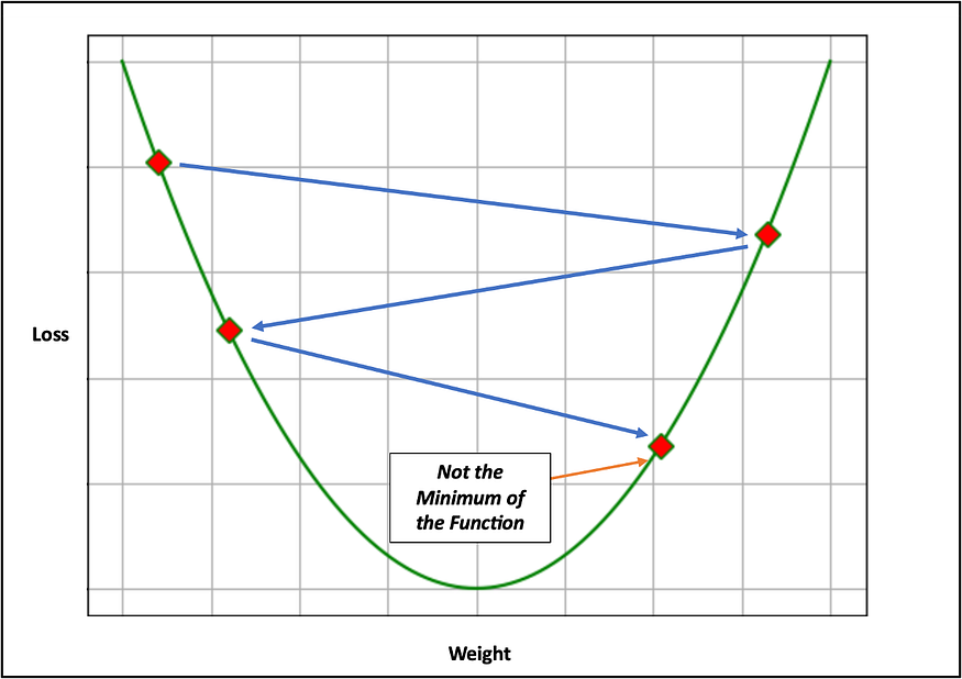
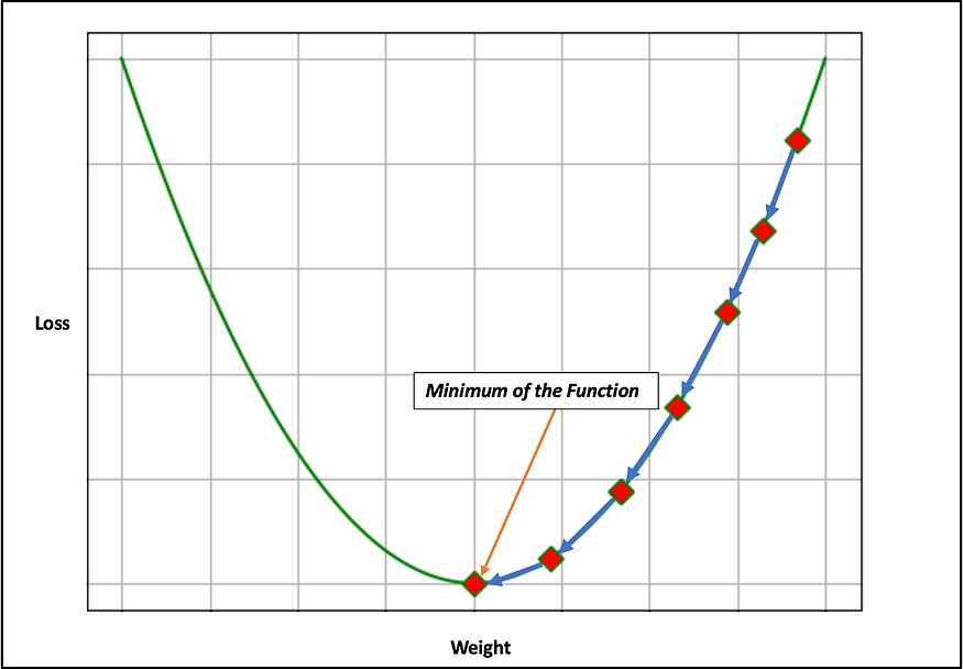
Gradient Descent: Using gradient descent, we can find the optimal prediction p ≈ y, by finding the minimum of the Loss function. In essence, we are trying to find the best weights that produce the lowest Loss function result.

Learning Rate: If we adjust each weight by a small amount, we can then assess how this will change the model’s prediction performance. The learning rate is an adjustable hyperparameter that we use to do this.

Intuitive examples of gradient descent have been provided below, using a large learning rate and a small learning rate. As shown in Fig. 26, the larger the learning rate, the faster the network is to train but it may never reach the minimum of the function (0). In Fig. 27 the smaller the learning rate, the longer it will take to train the network, but more likely to get closer to the minimum of the function.

Note: Common values for learning rates are 0.1 or 0.01 but can be adjusted/explored during network training.

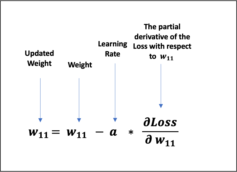
Updating the weights using the gradient descent algorithm :

We use the gradient descent algorithm to update the model’s weights during each training iteration.

An intuitive example of updating one weight for one iteration has been provided below. In this example, we multiply the partial derivative of the Loss with respect to weight (w11) by the learning rate (a). We reduce the weight (w11) by this value. This produces the new w11 weight used in the next iteration of the neural network.

For our neural network, we will use 100,000 iterations and a learning rate of 0.1( 1e-1). This means our weights will be initialised and then updated 99,999 times, with each iteration using a learning rate of 0.1. Each iteration includes all 4 training examples. As mentioned above, we can adjust these hyperparameters to optimise the model’s predictions.

A flow chart demonstrating the optimization process has been provided in Fig. 29. As shown, the weights are iteratively updated. For each iteration, the Cost function shows the average difference across all training examples until the final model predictions are produced (in our case, at iteration 100,000 ).

Important Note: As mentioned at the beginning of this article we have only trained the MLP. In reality, after training has been completed, the weights of a model would be frozen. The model would then be evaluated on unseen test data to assess how well it generalises.

Summary:

We have explored the MLP from a mathematical and visual perspective, covering forward propagation, backpropagation, and optimization. An overview of the key steps relating to model training has been visualized in Fig. 30:

For the purposes of this article and the simple problem it attempted to address, we have used a specific activation function, optimization algorithm, and Loss/Cost function. In other scenarios, where the data is much larger and more complex, these choices might not be the most suitable. Although not exhaustive, I have listed additional activation functions, optimization algorithms, and Loss/Cost functions below, which I urge the reader to explore and compare to what has been used in this article!

Activation Functions:

• Rectified Linear Unit (ReLU)
• Leaky Rectified Linear Unit (LReLU)
• Tanh Function

Optimization Algorithms :

• Stochastic Gradient Descent
• Mini Batch Gradient Descent
• Adaptive Moment Estimation (Adam)

Loss/Cost Functions:

• Mean Squared Error (MSE)
• Mean Absolute Error (MAE)
• Categorical Cross-Entropy Loss

The Code :

The following code implements the MLP based on the XOR training data discussed above:

#import required libaries
import numpy as np
from matplotlib import pyplot as plt

class MLP():

“””
This is the MLP class used to feedforward and backpropagate the network across a defined number
of iterations and produce predictions. After iteration the predictions are assessed using
Binary Cross Entropy Cost function.
“””

print(‘Running…’)

def __init__(self, design_matrix, Y, iterations=100000, lr=1e-1, input_layer = 2, hidden_layer = 3,output_layer =1):
self.design_matrix = design_matrix #design matrix attibute
self.iterations = iterations #iterations attibute
self.lr = lr #learning rate attibute
self.input_layer = input_layer #input layer attibute
self.hidden_layer = hidden_layer #hidden layer attibute
self.output_layer = output_layer #output layer attibute
self.weight_matrix_1 = np.random.randn(self.input_layer, self.hidden_layer) #weight attribute connecting to the hidden layer
self.weight_matrix_2 = np.random.randn(self.hidden_layer, self.output_layer)#weight attribute connecting to the output layer
self.cost = [] #cost list attribute
self.p_hats = [] #predictions list attribute

def sigmoid(self, x): # sigmoid function used at the hidden layer and output layer
return 1 / (1 + np.exp(-x))

def sigmoid_derivative(self, x): # sigmoid derivative used for backpropgation
return self.sigmoid(x) * (1 – self.sigmoid(x))

def forward_propagation(self):#define function to feedforward the network
z = np.dot(self.design_matrix, self.weight_matrix_1) #linear transformation to the hidden layer
activation_func = self.sigmoid(z)#hidden layer activation function
zh = np.dot(activation_func, self.weight_matrix_2)#linear transformation to the output layer
p_hat = self.sigmoid(zh)#output layer prediction
return z, activation_func, zh, p_hat

def BCECost(self, y, p_hat): # binary cross entropy cost function
bce_cost = -(np.sum(y * np.log(p_hat) + (1 – y) * np.log(1 – p_hat))) / len(y)
return bce_cost

def backword_prop(self, z_1, activation_func, z_2, p_hat): #backpropagation
del_2_1 = p_hat – Y
partial_deriv_2 = np.dot(activation_func.T, del_2_1) #∂loss/∂p *∂p/∂zh * ∂zh/∂wh
del_1_1 = del_2_1
del_1_2 = np.multiply(del_1_1, self.weight_matrix_2.T)
del_1_3 = np.multiply(del_1_2, self.sigmoid_derivative(z_1))
partial_deriv_1 = np.dot(self.design_matrix.T, del_1_3) #∂loss/∂p * ∂p/∂zh * ∂zh/∂h * ∂h/∂z * ∂z/∂w
return partial_deriv_2, partial_deriv_1

def train(self):#train the network
for i in range(self.iterations): #loop based on number of iterations
z_1, activation_func, z_2, p_hat = self.forward_propagation()# feedforward
partial_deriv_2, partial_deriv_1 = self.backword_prop(z_1, activation_func, z_2, p_hat)#backpropgate
self.weight_matrix_1 = self.weight_matrix_1 – self.lr * partial_deriv_1#update weights connecting to the hidden layer (gradient descent)
self.weight_matrix_2 = self.weight_matrix_2 – self.lr * partial_deriv_2#update weights connecting to the output layer (gradient descent )
self.cost.append(self.BCECost(Y, p_hat))#store BCE cost in list
self.p_hats.append(p_hat)#store predictions in list

print(‘Training Complete’)
print(‘—————————————————————————-‘)

# Prepare the XOR Logic Gate data: create an array for each training example x feature, and an array for each corrosponding y label.
X = np.array([[1, 0], [0, 1], [0, 0], [1, 1]]) #input features (4 x 2 design matrix)
Y = np.array([[1], [1], [0], [0]])#ground truth y labels (4×1)

mlp = MLP(X,Y)#Pass data to the model (design matrix and y label)
mlp.train() #Train the model

#plot the cost function
plt.grid()
plt.plot(range(mlp.iterations),mlp.cost)
plt.xlabel(‘Iterations’)
plt.ylabel(‘Cost’)
plt.title(‘BCE Cost Function’)

#Print predictions, number of iterations and the ground truth labels.
print(f’\n The MLP predictions for each training example, based on {mlp.iterations} iterations are:\n\n{np.round(mlp.p_hats[-1],2)}’)
print(‘\n—————————————————————————-‘)
print(f’\n The ground truth Y labels are are:\n\n{Y}’)

As shown above, the model’s Cost function has reduced as the training iterations have increased. The Cost function is close to 0, meaning our predictions are close to our ground truth labels!

Run the code yourself and try adjusting the learning rate and a number of training iterations to see what happens.

Special thanks to Mate Dénes for their feedback and review.

 

Join thousands of data leaders on the AI newsletter. Join over 80,000 subscribers and keep up to date with the latest developments in AI. From research to projects and ideas. If you are building an AI startup, an AI-related product, or a service, we invite you to consider becoming a sponsor.

Published via Towards AI