


Temporal Edge Regression with PyTorch Geometric
Last Updated on November 5, 2023 by Editorial Team
Author(s): Marco Lomele
Originally published on Towards AI.
Graphs and Time
Graphs are becoming one of the favorite tools of data scientists. Their inherent structure allows for efficient storage of complex information, such as the ongoing protein interactions in your body or the ever-evolving social network surrounding you and your friends.
Additionally, graphs can be adapted to temporal scenarios. They can vary from the simple static form, where there is no notion of time, to a fluid spatiotemporal setup, where the topology is fixed but the features change at regular intervals, to the chaotic, fully continuous and time-dynamic mode, where everything can change at any time. [1]
Graph Neural Networks (GNNs) are used to process graphs, and many have already demonstrated exceptional results for recommendation systems, supply chain optimization, and road traffic prediction. [2] Nonetheless, most GNNs operate on static graphs, limiting their use for temporal problems.
What happens then when we have time series data stored within graphs for which we want to predict future values? It turns out that the Transformer could be a solution, as it has already shown remarkable performance in time series forecasting scenarios. [3]
Our Goal
To study the effectiveness of combining GNNs and Transformers for time series forecasting on graphs, we will be solving an edge weight prediction problem. Using the data provided by Vesper, we will create a sequence of spatio-temporal graphs acting as snapshots of the global trade market of butter. Our goal is then to
forecast worldwide butter trade volumes for the next three months.
Trade Data
All countries publish their trade records on a monthly basis. Each record indicates the reporting country, the partner country in the transaction, the product, and its traded volume (our target variable). Since each trade is logged twice, we focus on exports.
The data at our disposal ranges from January 2015 to April 2023, totaling more than 153,000 transactions. The dataset lists 242 “countries,” including the exports of regions that aggregate multiple countries together, which means that there are 242*241 = 58,322 possible country pairs. Across all months, each pair is an individual time series that we will be forecasting.
We also include other data series as features to support our model’s learning. In particular, we define country-specific features, such as domestic butter production or GDP, and pair-specific attributes, such as the traded volume or the exchange rate.
Building Graphs with PyTorch Geometric
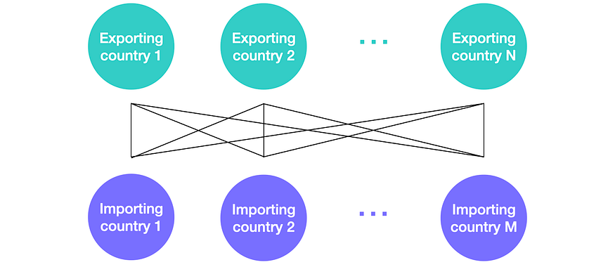
We proceed by segmenting the data monthly. We designate two types of nodes: one for the exporter (exp_id) and another for the importer (imp_id). Undirected edges are then used to indicate the relationship between two countries.
In this manner, we can assign distinct country-specific features to the various types of nodes and embed the pair-specific attributes on the edges. The resulting graph for each month is heterogeneous, fully connected, and bipartite. It can be visualized as follows.
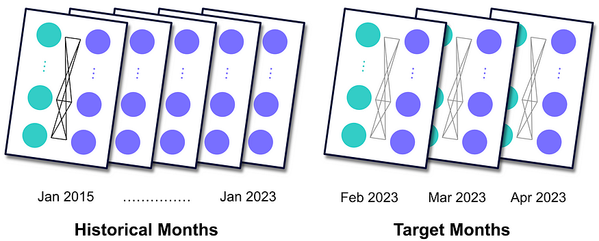
Altogether, we end up with a sequence of graphs, each serving as a static snapshot of the market’s status at the end of a specific month. Assuming that the data series for the features are updated more rapidly compared to trade data, we can create graphs for the three most recent months we aim to predict, which we refer to as the target months. These graphs are identical to the historical months but lack trade information in the edges.
In Python, we construct a heterogeneous graph using the HeteroData object from the PyTorch Geometric (PyG) library. [4]
!pip install torch_geometric

import torch
from torch_geometric.data import HeteroData
from torch_geometric.transforms import ToUndirected

def generate_monthly_snapshot(monthly_data):
 """
 Generate a HeteroData object as snapshot of one month.

 Args:
 monthly_data (list): List of pandas dataframes with trade
 and features' data for one month.

 Returns:
 HeteroData: Object containing node features and edge attributes.
 """
 monthly_snp = HeteroData()

 # Ingesting the data
 trade_figs = monthly_data[0]
 exporters_features = monthly_data[1]
 importers_features = monthly_data[2]
 edge_attrs = monthly_data[3]

 # Creating the nodes
 exp_ids = trade_figs['exp_id'].unique(),
 exp_ids = torch.from_numpy(exp_ids).to(torch.int64)

 exporters_ftrs_arr = exporters_features.values
 exporters_ftrs_arr = np.vstack(exporters_ftrs_arr).astype(np.float64)

 exporters_ftrs_tensor = torch.tensor(exporters_ftrs_arr,
 dtype=torch.float)
 monthly_snp['exp_id'].x = exporters_ftrs_tensor

 imp_ids = trade_figs['imp_id'].unique(),
 imp_ids = torch.from_numpy(imp_ids).to(torch.int64)

 importers_ftrs_arr = importers_features.values
 importers_ftrs_arr = np.vstack(importers_ftrs_arr).astype(np.float64)

 importers_ftrs_tensor = torch.tensor(importers_ftrs_arr,
 dtype=torch.float)
 monthly_snp['imp_id'].x = importers_ftrs_tensor

 # Creating the edges
 edge_index = torch.stack([
 torch.tensor(trade_figs['exp_id'].values, dtype=torch.long),
 torch.tensor(trade_figs['imp_id'].values, dtype=torch.long)],
 dim=0)

 monthly_snp['exp_id', 'volume', 'imp_id'].edge_index = edge_index

 vol = torch.from_numpy(trade_figs['volume'].values).to(torch.float)
 monthly_snp['exp_id', 'volume', 'imp_id'].edge_label = vol

 edge_attrs_arr = edge_attrs.values
 edge_attrs_arr = np.vstack(edge_attrs_arr).astype(np.float64)
 edge_attrs_tensor = torch.tensor(edge_attrs.values).to(torch.float)
 monthly_snp['exp_id',
 'volume', 'imp_id'].edge_attrs = edge_attrs_tensor

 monthly_snp['exp_id', 'volume',
 'imp_id'].edge_label_index = monthly_snp['exp_id',
 'volume','imp_id'].edge_index.clone()

 monthly_snp = ToUndirected()(monthly_snp)
 del monthly_snp[('imp_id',
 'rev_volume', 'exp_id')]['edge_label']

 return monthly_snp
Note that trade volume data is stored in variable vol, and it is assigned to the edge weights, called edge_label in PyG, instead of the edge attributes. The resulting HeteroData object for January 2015 is:
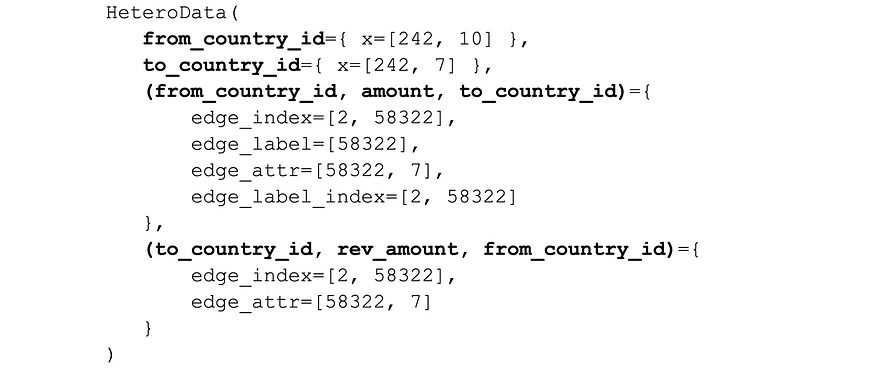
It contains the following variables:
- exp_id: a list of node features per exporting node.
- imp_id: a list of node features per importing node.
- edge_index: a list of node indices denoting the connections of the edges.
- edge_label: a list of the edge labels, where our target variable is stored.
- edge_label_index: a list mirroring edge_index, for the edge labels.
- edge_attr: a list of edge attributes per edge.
With the graphs ready, we can proceed to define the individual components of our model.
The Model — Individual Components
Taking inspiration from the time-and-graph approach, we employ an Encoder-Decoder architecture. [5] The three crucial units are:
- GNN Encoder: to generate static node embeddings.
- Transformer: to create temporal node embeddings.
- Edge Decoder: to extrapolate predictions.
GNN Encoder
Similar to how Convolutional Neural Networks work with images, GNNs perform an optimizable transformation on all the features of a graph, preserving the data distributions within that graph. [6] They are used to convert a complex graph schema into vectors of numbers known as node embeddings. Naturally, some information loss is unavoidable. Therefore, the better the GNN, the lower the loss. For more information on GNNs, you can refer to this Medium article.
In our case, we deploy the GATv2Conv operator, which introduces attention to rank neighboring nodes based on their significance in creating each node embedding. [7] In Python:
import torch.nn as nn
import torch.nn.functional as F
from torch_geometric.nn import GATv2Conv
from torch.nn import BatchNorm

class GNNEncoder(nn.Module):
 """
 GNN Encoder module for creating static node embeddings.

 Args:
 hidden_channels (int): The number of hidden channels.
 num_heads_GAT (int): The number of attention heads.
 dropout_p_GAT (float): Dropout probability.
 edge_dim_GAT (int): Dimensionality of edge features.
 momentum_GAT (float): Momentum for batch normalization.
 """

 def __init__(self, hidden_channels, num_heads_GAT,
 dropout_p_GAT, edge_dim_GAT, momentum_GAT):

 super().__init__()

 self.gat = GATv2Conv((-1, -1), hidden_channels,
 add_self_loops=False, heads=num_heads_GAT,
 edge_dim=edge_dim_GAT)

 self.norm = BatchNorm(hidden_channels, momentum=momentum_GAT,
 affine=False, track_running_stats=False)

 self.dropout = nn.Dropout(dropout_p_GAT)

 def forward(self, x_dict, edge_index, edge_attrs):
 """
 Forward pass of the GNNEncoder.

 Args:
 x_dict (torch.Tensor): node types as keys and node features
 for each node as values.
 edge_index (torch.Tensor): see previous section.
 edge_attrs (torch.Tensor): see previous section.

 Returns:
 torch.Tensor: Static node embeddings for one month.
 """
 x_dict = self.dropout(x_dict)
 x_dict = self.norm(x_dict)
 nodes_embedds = self.gat(x_dict, edge_index, edge_attrs)
 nodes_embedds = F.leaky_relu(nodes_embedds, negative_slope=0.1)
 return nodes_embedds
Transformer
Transformers are a remarkable architecture capable of making sequence-to-sequence predictions and serve as the foundation of large language models like ChatGPT. [8] Through complex attention mechanisms, they can quantify the relationships of embeddings relative to input order. Then, they generate a relevant prediction (as an embedding) for the next element in the sequence. To understand Transformers on a deeper level, I recommend this YouTube video.
We implement a transformer to extrapolate the temporal dynamics across the static monthly snapshots and generate a “temporal” node embeddings for the month under prediction. After applying positional encoding, as shown on PyTorch’s website, we define:
class Transformer(nn.Module):
 """
 Transformer-based module for creating temporal node embeddings.

 Args:
 dim_model (int): The dimension of the model's hidden states.
 num_heads_TR (int): The number of attention heads.
 num_encoder_layers_TR (int): The number of encoder layers.
 num_decoder_layers_TR (int): The number of decoder layers.
 dropout_p_TR (float): Dropout probability.
 """

 def __init__(
 self, dim_model, num_heads_TR, num_encoder_layers_TR,
 num_decoder_layers_TR, dropout_p_TR):

 super().__init__()

 self.pos_encoder = PositionalEncoding(dim_model)
 self.transformer = nn.Transformer(
 d_model=dim_model,
 nhead=num_heads_TR,
 num_decoder_layers=num_encoder_layers_TR,
 num_encoder_layers=num_decoder_layers_TR,
 dropout=dropout_p_TR)

 def forward(self, src, trg):
 """
 Forward pass of the Transformer module.

 Args:
 src (torch.Tensor): Input sequence with dimensions
 (seq_len, num_of_nodes, node_embedds_size).
 trg (torch.Tensor): Last element of src, with dimensions
 (1, num_of_nodes, node_embedds_size).

 Returns:
 torch.Tensor: Temporal node embeddings for the month
 under prediciton.
 """
 src = self.pos_encoder(src)
 trg = self.pos_encoder(trg)
 temporal_node_embeddings = self.transformer(src, trg)
 return temporal_node_embeddings
Edge Decoder
This unit receives the temporal node embeddings and makes inferences for the target variable. In practice, the embeddings are passed through two linear layers that reduce the dimensionality of a pair of node embeddings to a single number: the predicted trade volume between a specific pair of countries. For a refresher on linear layers, I invite you to read this Medium article.
class EdgeDecoder(nn.Module):
 """
 Edge Decoder module to infer the predictions.

 Args:
 hidden_channels (int): The number of hidden channels.
 num_heads_GAT (int): The number of attention heads in GAT layer.
 """

 def __init__(self, hidden_channels, num_heads_GAT):

 super().__init__()

 self.lin1 = nn.Linear(2 * hidden_channels * num_heads_GAT,
 hidden_channels)
 self.lin2 = nn.Linear(hidden_channels, 1)

 def forward(self, z_dict, edge_label_index):
 """
 Forward pass of the EdgeDecoder module.

 Args:
 z_dict (dict): node type as keys and temporal node embeddings
 for each node as values.
 edge_label_index (torch.Tensor): see previous section.

 Returns:
 torch.Tensor: Predicted edge labels.
 """
 row, col = edge_label_index

 z = torch.cat([z_dict['exp_id'][row], z_dict['imp_id'][col]],
 dim=-1)
 z = self.lin1(z)
 z = F.leaky_relu(z, negative_slope=0.1)
 z = self.lin2(z)
 return z.view(-1)
The Model — All Together
The full model is initialized as follows:
# Any HeteroData object, needed for model initialization.
hetero_data_init = monthly_data[0]

device = torch.device('cuda' if torch.cuda.is_available() else 'cpu')

hidden_channels = 32

num_heads_GAT = 4
dropout_p_GAT = 0.3
edge_dim_GAT = 7
momentum_GAT = 0.1

num_heads_TR = 4
num_encoder_layers_TR = 2
num_decoder_layers_TR = 2
dropout_p_TR = 0.3

model = Model(hidden_channels=hidden_channels,
 num_heads_GAT=num_heads_GAT,
 dropout_p_GAT=dropout_p_GAT,
 edge_dim_GAT=edge_dim_GAT,
 momentum_GAT=momentum_GAT,
 num_heads_TR=num_heads_TR,
 num_encoder_layers_TR=num_encoder_layers_TR,
 num_decoder_layers_TR=num_decoder_layers_TR,
 dropout_p_TR=dropout_p_TR).to(device)
To understand how the model is constructed and the interplay between the three units, I will guide you through the training process of one epoch. After setting the number of months to predict (3 in our case) and choosing the optimizer with its learning rate (Adam, 0.00005), we run:
for epoch in range(1, epochs + 1):

 # Train phase
 for m in range(5, tot_num_months - num_predicting_months):
 m_lag4 = monthly_snapshots_list[m - 4]
 m_lag3 = monthly_snapshots_list[m - 3]
 m_lag2 = monthly_snapshots_list[m - 2]
 m_lag1 = monthly_snapshots_list[m - 1]
 m = monthly_snapshots_list[m]

 m_lag4 = m_lag4.to(device)
 m_lag3 = m_lag3.to(device)
 m_lag2 = m_lag2.to(device)
 m_lag1 = m_lag1.to(device)
 m = m.to(device)

 historical = [m_lag4, m_lag3, m_lag2, m_lag1]

 train_loss = train(historical, m)
 train_pred, train_target, train_rmse = test(historical, m)
Here, monthly_snapshots_list is the sequence of monthly snapshots, and tot_num_months equals its length. To capture the temporal trends, we implicitly set in range(5, …) a window with a horizon of 4. This setup ensures that historical always holds the four months leading up to the month under prediction, named m. During training, we slide this window along the sequence of monthly snapshots, updating m with each iteration.
For the train and test functions, we follow a typical structure inspired by the “Training a Heterogeneous GNN” section of this Google Colab notebook. The functions send historical and m to the model, which is initialized in its complete form like this:
class Model(nn.Module):
 """
 The complete model.

 Args:
 See previous code snippets.
 """

 def __init__(self, hidden_channels, num_heads_GAT, dropout_p_GAT,
 edge_dim_GAT, momentum_GAT, num_heads_TR,
 num_encoder_layers_TR, num_decoder_layers_TR,
 dropout_p_TR):

 super().__init__()

 self.encoder = GNNEncoder(hidden_channels, num_heads_GAT,
 dropout_p_GAT, edge_dim_GAT,
 momentum_GAT)

 self.encoder = to_hetero(self.encoder,
 metadata=hetero_data_init.metadata(),
 aggr='sum')

 self.transformer = Transformer(hidden_channels * num_heads_GAT,
 num_heads_TR,
 num_encoder_layers_TR,
 num_decoder_layers_TR, dropout_p_TR)

 self.decoder = EdgeDecoder(hidden_channels, num_heads_GAT)
The to_hetero function adapts the GATv2Conv operator to heterogeneous graphs. Next, we define the forward pass, summarised by the following diagram:
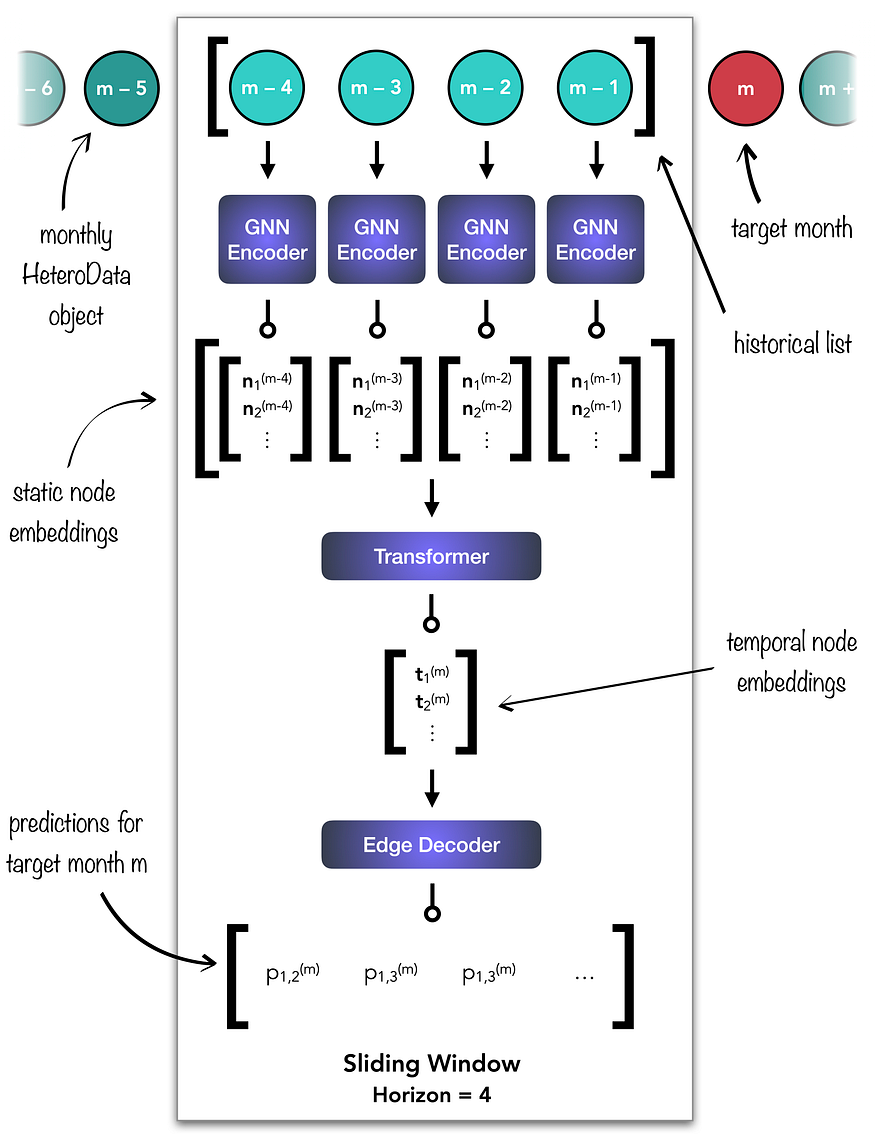
First, each HeteroData object from the historical list is passed through the GNN Encoder. Next, the resulting static node embeddings are concatenated into the source tensor for the Transformer. The unit generates the temporal node embeddings for the month under prediction, which are subsequently fed to the Edge Decoder. The latter ultimately produces the predictions for month m. In Python:
def forward(self, historical, m):
 """
 Forward pass of the Model.

 Args:
 See previous code snippets.

 Returns:
 torch.Tensor: Predicted edge labels for the month
 under prediciton, m.
 """

 # GNN Encoder
 embedds_static_list = []
 for month in historical:
 x_dict = month.x_dict
 edge_index_dict = month.edge_index_dict
 edge_attrs_dict = month.edge_attrs_dict
 edge_label_index = month['exp_id',
 'volume', 'imp_id'].edge_label_index

 z_dict_month = self.encoder(x_dict,
 edge_index_dict, edge_attrs_dict)

 num_exp_nodes = z_dict_month['exp_id'].size()[0]
 num_imp_nodes = z_dict_month['imp_id'].size()[0]

 month_embedds = torch.cat((z_dict_month['exp_id'],
 z_dict_month['imp_id']), 0)

 embedds_static_list.append(month_embedds)

 embedds_static = torch.stack(embedds_static_list)

 # Transformer (with positional encoding)
 src = embedds_static
 trg = embedds_static_list[3]
 trg = trg.unsqueeze(0)
 embedds_temp = self.transformer(src, trg)

 embedds_temp = embedds_temp.squeeze(0)
 embedds_exp, embedds_imp = embedds_temp.split([num_exp_nodes,
 num_imp_nodes],
 dim=0)

 # Prepare input for Edge Decoder.
 z_dict_m_temp = {'exp_id': embedds_exp,
 'imp_id': embedds_imp}
 edge_label_index = m['exp_id', 'volume', 'imp_id'].edge_label_index

 # Edge Decoder
 edge_label_pred_m = self.decoder(z_dict_m_temp, edge_label_index)
 return edge_label_pred_m
For each training step, we compute the Mean Squared Error by comparing the model’s forecast to the actual trade volumes of the month under prediction. The loss is then back-propagated to each unit, with PyTorch ensuring that this occurs in a balanced manner.
At the end of the training phase, we slide the window once more and allow the model to compute the predictions for the first month in the target list. When the window is moved again, the historical list includes the last three training months plus the first target month, which has just been enriched with the predicted trade volumes. Therefore, as we slide the window into the future, the model will increasingly base of its forecasts on previous predictions it made.
After training our model for several epochs, we proceed to its evaluation.
The Results
To assess the effectiveness of our model, we benchmark its performance against traditional forecasting techniques by running PyCaret forecasting experiments on a subset of trade routes. [9] The model achieves perfect predictions for when trade doesn’t occur, and performs relatively well on pairs with extremely high volumes. Both scenarios involve trades of outlying amounts, making their predictions easier to make. In contrast, trade routes with average volumes are more challenging to distinguish, explaining the model’s inconsistent performance in such cases.
Future developments will focus on enhancing the model’s ability to capture the complexity within the data by:
- expanding the set of features;
- optimizing the architecture and hyperparameters;
- exploring methods from the PyG Temporal library;
- increasing the size of the training and testing datasets. [10]
The Verdict
In this article, we created a sequence of static heterogeneous graphs to represent the global trade market of butter. We then implemented a model that slides along that sequence and uses a Graph Neural Network and a Transformer to extrapolate relationships within and across snapshots. Finally, we tested the model’s performance against traditional forecasting methods to quantify its relative improvement.
Given the size of the problem and the various facets of improvement we discussed, it is premature to draw a conclusion on the effectiveness of combining GNNs with Transformers for making time series predictions on graphs.
However, graphs have demonstrated their strength in representing temporal problems. Due to their holistic nature, they allowed us to learn relationships between pairs of nodes by drawing insights from other pairs, which becomes useful in the future if the graph structure changes. In contrast, traditional forecasting methods work on an individual series completely in isolation and lack this advantage.
For those interested in the full story of the butter trade challenge, feel free to read this other Medium article that I wrote. If this article has inspired you and helped you to better understand time series forecasting on graphs, I invite you to connect with me on LinkedIn!
Acknowledgments
Data provided by Vesper, the most comprehensive and user-friendly commodity intelligence platform. Project ideator: Ea Werner.
Bibliography
- Machine Learning on Dynamic Graphs and Temporal Graph Networks U+007C MLSYS 2021. (n.d.). YouTube. https://youtube.com/watch?v=xzcYyIiFXcY&list=PLG2m1ulw_f2Xz4FIVR0Bcuew8sZ%20S9hm-z&index=1
- Zhou, J. (2018, December 20). Graph Neural Networks: A Review of Methods and Applications. arXiv.org. https://arxiv.org/abs/1812.08434
- Yes, Transformers are Effective for Time Series Forecasting (+ Autoformer). (n.d.). https://huggingface.co/blog/autoformer
- Home — PYG. (n.d.). https://pyg.org/
- Huang. (2023, January 19). Temporal Graph Learning in 2023 — Towards Data Science. Medium. https://towardsdatascience.com/temporal-graph-learning-in-2023-d28d1640dbf2#a31b
- Labonne, M. (n.d.). Hands-on graph Neural networks using Python. O’Reilly Online Learning. https://www.oreilly.com/library/view/hands-on-graph-neural/9781804617526/
- Brody, S. (2021, May 30). How Attentive are Graph Attention Networks? arXiv.org. https://arxiv.org/abs/2105.14491
- Vaswani, A. (2017, June 12). Attention is all you need. arXiv.org. https://arxiv.org/abs/1706.03762
- Home — PyCaret. (2023, June 28). PyCaret. https://pycaret.org/
- PyTorch Geometric Temporal Documentation — PyTorch Geometric Temporal documentation. (n.d.). https://pytorch-geometric-temporal.readthedocs.io/
Join thousands of data leaders on the AI newsletter. Join over 80,000 subscribers and keep up to date with the latest developments in AI. From research to projects and ideas. If you are building an AI startup, an AI-related product, or a service, we invite you to consider becoming a sponsor.
Published via Towards AI
Towards AI Academy
We Build Enterprise-Grade AI. We'll Teach You to Master It Too.
15 engineers. 100,000+ students. Towards AI Academy teaches what actually survives production.
Start free — no commitment:
→ 6-Day Agentic AI Engineering Email Guide — one practical lesson per day
→ Agents Architecture Cheatsheet — 3 years of architecture decisions in 6 pages
Our courses:
→ AI Engineering Certification — 90+ lessons from project selection to deployed product. The most comprehensive practical LLM course out there.
→ Agent Engineering Course — Hands on with production agent architectures, memory, routing, and eval frameworks — built from real enterprise engagements.
→ AI for Work — Understand, evaluate, and apply AI for complex work tasks.
Note: Article content contains the views of the contributing authors and not Towards AI.
Related posts
Recent Posts

")


