


Tackling Imbalanced Data Using imbalanced-learn, Part 1: Under-Sampling
Last Updated on July 17, 2023 by Editorial Team
Author(s): Christian Kruschel
Originally published on Towards AI.
In the field of machine learning, working with imbalanced datasets can present a significant challenge. Imbalanced data occurs when the distribution of classes in the dataset is uneven, with one class being dominant compared to the others. This can lead to biased models that perform poorly on the minority class. In this article, we will explore how to address imbalanced data using the Road Accidents UK dataset and the imbalanced-learn Python package.
This is the first article in a series of four; it considers the topic of Undersampling, which will be defined later. The crucial idea of this series is to derive an intuition when the considered methods can help. With this study, we will learn the best undersampling methods, which to choose to improve which class, and for which purpose the classifier should be constructed.
This article will first define basic concepts, the considered dataset, and the experiment setup. Thereafter, the most popular methods will be introduced and applied to the experimental setup. In the end, the results of all methods are compared via different metrics.
What is Imbalanced Data?
Imbalanced data refers to datasets where the classes are not represented equally. In the case of the Road Accidents UK dataset, it contains information about road accidents, including various attributes such as location, time, weather conditions, and severity of the accidents. However, the occurrence of severe accidents is relatively rare compared to minor accidents, resulting in an imbalanced dataset. When training a machine learning model on imbalanced data, the model tends to favor the majority class, leading to poor performance for the minority class. In the case of the Road Accidents UK dataset, this means that a model trained on the original dataset would likely struggle to accurately predict severe accidents.
Road Accidents in the UK
The Road Safety Data dataset provides detailed information about road accidents in the United Kingdom, including factors such as date, time, location, road type, weather conditions, vehicle types, and accident severity. It is a valuable resource for analyzing and understanding the causes and patterns of road accidents. The dataset is available at [01]; in this article, we are considering the data from 2021.
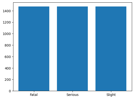
Three different tables are available describing information about injured individuals, vehicle characteristics, and accident conditions. The dataset can be merged via their accident_index. For prediction, we consider the information about accident_severity. Accidents can be slight, serious, or fatal. The following histogram shows how much data for all three classes is available.
As 77% of all accidents are slight and 1.4% are fatal, this is an imbalanced category and any vanilla classifier will have an accuracy of exactly 77% as it only estimates an accident is slight.

Addressing Imbalanced Data with imbalanced-learn
imbalanced-learn [02] is a Python package specifically designed to address the challenges posed by imbalanced data. It provides various techniques for resampling the data, which can help balance the class distribution and improve model performance. Let’s explore a few of these techniques.
- Under-Sampling: This involves randomly removing samples from the majority class to match the number of samples in the minority class. This technique can help create a more balanced dataset, but it may result in loss of information if the removed samples contain important patterns.
- Over-Sampling: This involves randomly duplicating samples from the minority class to increase its representation in the dataset. This technique helps prevent information loss but can also lead to overfitting if not used carefully.
- Combination of over- and under-sampling methods
In this article, we will focus on Under-Sampling techniques. The other methods will be considered in future articles.
Experiment Setup
For demonstrating the methods in imbalanced learn, we consider a fixed neural network that will be trained with the same initialization. Twenty-six features are selected, and a feed-forward network with one hidden layer and 15 neurons is trained.
from sklearn.model_selection import train_test_split
from sklearn.preprocessing import StandardScaler
from tensorflow.keras.models import Sequential
from tensorflow.keras.layers import Dense

X_train, X_test, y_train, y_test = train_test_split(X_input, y_input, test_size=0.2, random_state=20)

scaler = StandardScaler()
scaler.fit(X_train)
X_transform = scaler.transform(X_train)

model = Sequential()
model.add(Dense(15, input_shape=(X_transform.shape[1],), activation='relu'))
model.add(Dense(3, activation='softmax'))

# Compile model
model.compile(loss='sparse_categorical_crossentropy', optimizer='adam', metrics=['accuracy'])
model.save_weights("weights.hf5")
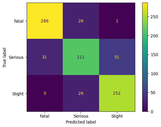
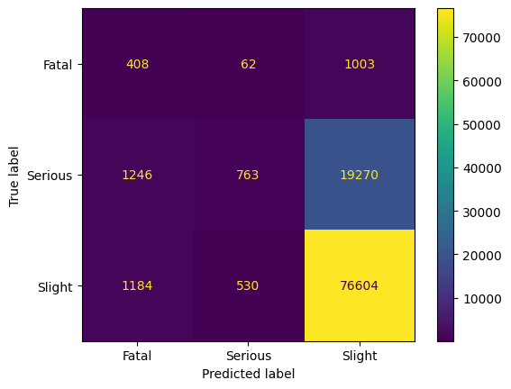
Note that the confusion matrix above was produced with this code. To guarantee comparability, the following will be repeated ten times. We will only consider accuracy as the performance metric.
import numpy as np

model.load_weights("weights.hf5")
history = model.fit(X_transform, y_train, epochs=60, verbose = 0)

_, x2 = model.evaluate(scaler.transform(X_test), y_test, verbose = 0)
print('Accuracy on randomly selected test data:', x2)

y_test_pred = np.argmax(model.predict(scaler.transform(X_test), verbose = 0))
In the following, violin plots are considered. Violin plots give a chance to compare different data distributions. In the graphic below, we see the distribution of the accuracy when the model is trained 10 times. The black box in the middle is part of the lower to the upper quantile of the accuracy data. The white dot is the median. The outer form of the plot is done by a kernel density estimation (KDE) of the model's accuracy. A good introduction can be found at [03].
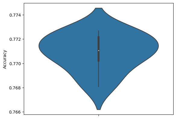
Note that the KDE plot is shown twice: left and right. When reducing the data, we will see different distributions on both sides: the full data and the reduced data.
Cluster Centroids with Mini-Batch K-Means
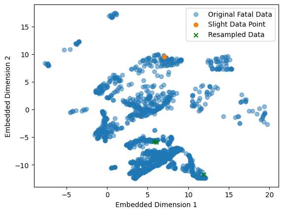
Cluster Centroids is a generation method, which means that it will generate synthetic data from the given. The data from the majority classes are fully removed by centroids of K-Means, i.e., here K-Means is applied with K = 1473 clusters. The following graphic gives an idea of what happened.

In this graphic, one can see the dimension reduction to 2D done by UMAP [09]. A good introduction is given in [10]. As the dimensionality is 26 in the original data, this plot can only give an idea of what is happening: Most point clouds are covered by centroids, and only a few outliers remain unseen in resampled data. From the idea of the algorithm, it is clear that the data is perfectly balanced. All classes have 1473 samples.
The results by the following code will be discussed in this section.
from sklearn.cluster import MiniBatchKMeans
from imblearn.under_sampling import ClusterCentroids

cc = ClusterCentroids(
 estimator=MiniBatchKMeans(n_init=10, random_state=0), random_state=42
)
X_res, y_res = cc.fit_resample(X_input, y_input)

X_train, X_test, y_train, y_test = train_test_split(X_res, y_res, test_size=0.2, random_state=20)

scaler = StandardScaler()
scaler.fit(X_train)
X_transform = scaler.transform(X_train)

for _ in range(10):
 model.load_weights("weights.hf5")
 history = model.fit(X_transform, y_train, epochs=60, verbose = 0)
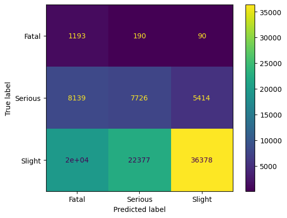
After training, we observe that we can train a good classifier on the reduced dataset. As the human intuition that there is an order in the classes, i.e., Slight < Serious < Fatal, we observe that the classifier has most problems with the neighboring class in this ordering. The precision for Fatal is above 90%. Hence, we have an excellent classifier for predicting Fatal, and still good classifier for the other classes. However, considering the trained model on the entire dataset gives a different insight.

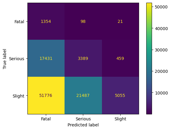
Applying the trained model on the entire dataset shows that mostly class Fatal is predicted; we see a clear bias to this class. The accuracy of the model is less than 10%; this model can not be used for any kind of analytics.
In conclusion, we saw that Centroid Cluster is an intuitive method for reducing the dataset with respect to balancing. In our example, the model can be used to analyze the minority class on the reduced dataset. However, the model has a very bad performance considering the entire dataset. This means, that resampled data does not represent the entire dataset. This might be due to a lot of outliers and missing data in the dataset but may also be the result of an imperfect balancing method. We will consider other balancing methods in the following.
Near Miss Undersampling
This method samples data from the majority classes, but will not generate synthetic data. It bases on the work [04] by Zhang and Mani in 2003 and uses the k-nearest neighbor method. Here, the average distance of a sample by the majority class with the k nearest neighbors of the minority class is considered. We sample from the majority by considering the smallest average distances.
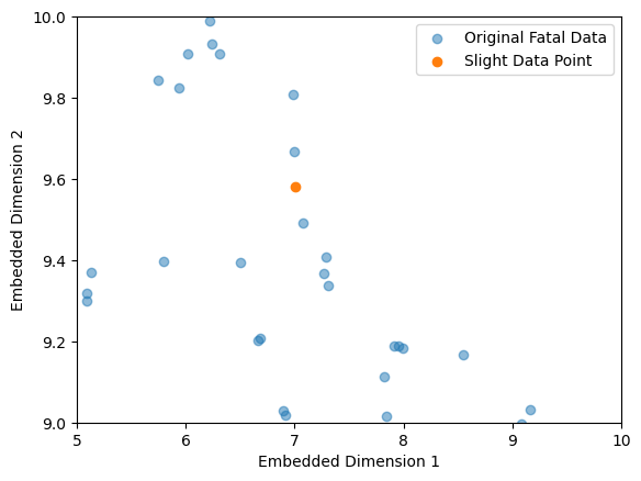
First, a K=3 nearest neighbor is trained on Fatal class data. That means, given a new sample, the nearest neighbor gives the three nearest Fatal data points as well as their distances to the Fatal data point. Hence, to each, say, Slight data point, three Fatal data points are given by nearest neighbor. Averaging over the 3 distances of each Slight data point brings us the Slight data ppoints which are the nearest to Fatal data. But, as UMAP is a distance-preserving dimensionality reduction, the graphic above shows that considering the eukledian distance is not a good idea at this data set.
A further version of Near Miss, version 2, considers the data points which are far away from the minority class. In general, this might be a good idea, as the nearest data points may be too close to the class boundary.
from imblearn.under_sampling import NearMiss

cc = NearMiss()
X_res, y_res = cc.fit_resample(X_input, y_input)

X_train, X_test, y_train, y_test = train_test_split(X_res, y_res, test_size=0.2, random_state=20)

scaler = StandardScaler()
scaler.fit(X_train)
X_transform = scaler.transform(X_train)

for _ in range(10):
 model.load_weights("weights.hf5")
 history = model.fit(X_transform, y_train, epochs=60, verbose = 0)
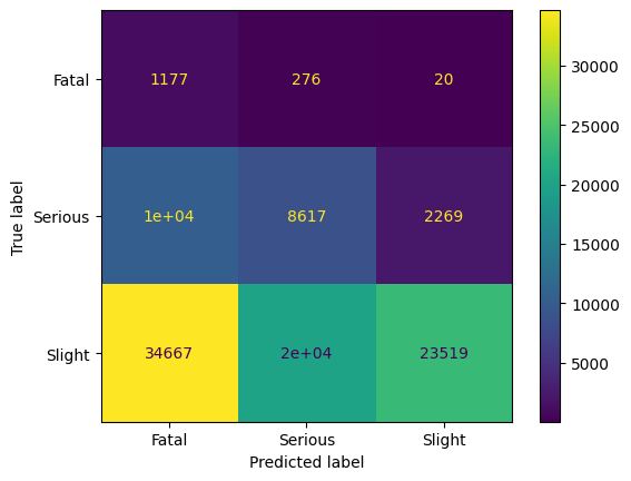
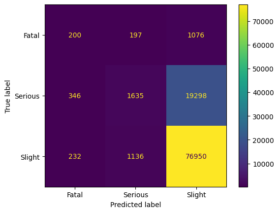
The code above uses the version with the smallest distance, version 1. Here also, both majority classes are reduced to 1472 samples. The accuracy decreases on the balanced dataset to 60%, but on the full dataset, the accuracy is 40%.
Considering Near Miss Version 2, we observe that it outperforms Version 1, especially in recall.
Instance Hardness Threshold

This is also a method where no synthetic data is generated. It is based on [05] by Smith, Martinez, and Giraud-Carrier in 2014. The authors studied 64 data sets with respect to samples where it is hard to classify correctly. In imbalanced-learn, it is done by training a classifier and getting the sample of the sample-only data that is good to classify. By default, the classifier is chosen as a Random Forest with 100 estimators. For each class, the samples were the prediction has the highest probabilities are chosen. This is done by considering the q-th percentile of the probabilities, with
q = 1 — #(samples in minority class)/#(samples in considered class).
Hence the dataset may not be sampled to the same size for all classes, but it is more balanced.
from imblearn.under_sampling import InstanceHardnessThreshold

cc = InstanceHardnessThreshold()
X_res, y_res = cc.fit_resample(X_input, y_input)

X_train, X_test, y_train, y_test = train_test_split(X_res, y_res, test_size=0.2, random_state=20)

scaler = StandardScaler()
scaler.fit(X_train)
X_transform = scaler.transform(X_train)

for _ in range(10):
 model.load_weights("weights.hf5")
 history = model.fit(X_transform, y_train, epochs=60, verbose = 0)
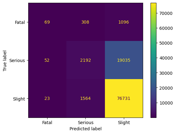
The idea may be judged as unfair as badly classified samples are deleted from the dataset. However, the idea is the same as by Near Miss, where the data close or far away from the class boundary is removed. It will be interesting if it helps to take only the best-classified samples.
Surprisingly, precision for class 2 increases
Edited Nearest-Neighbor Rule / All k-NN
Edited Nearest-Neighbor (ENN) based on [06] by Wildon in 1972 and also locates nearest neighbors of samples that are misclassified. The main idea is to apply the k-nearest neighbor, where k=3, to misclassified data points. Correctly classified samples remain. All kNN is an extension of ENN published in 1976 [07] by Tomek, where in an iteration, all misclassified samples are deleted. This leads to a confusing result in the following graphic: Many samples from the Slight class are classified correctly by the nearest neighbor method.

The fatal class remains in its size, while in the Slight class, only 20.000 samples are removed. By 1148 samples, the Serious class is now smaller than the Fatal class.
from imblearn.under_sampling import AllKNN

cc = AllKNN()
X_res, y_res = cc.fit_resample(X_input, y_input)

X_train, X_test, y_train, y_test = train_test_split(X_res, y_res, test_size=0.2, random_state=20)

scaler = StandardScaler()
scaler.fit(X_train)
X_transform = scaler.transform(X_train)

for _ in range(10):
 model.load_weights("weights.hf5")
 history = model.fit(X_transform, y_train, epochs=60, verbose = 0)
As we do not see improvements in the model performance, we focus on the last undersampling method from 2001.
Neighbourhood Cleaning Rule
This method by Laurikkala from 2001 [08] is a modification of Edited Nearest Neighbor (ENN). First, a 3-nearest neighbor is trained, and misclassified samples are removed if it belongs to the majority class. If the sample belongs to the minority class, the 3 closest samples to the majority class are removed.

Tomek Links
The last method we consider is Tomek Links. The author proposed in [07] that samples at the class boundary are removed. Here a Tomek link is a pair of samples, (a, b), with a and b in different classes, if there is no sample c such that for a distance d that d(a,c) < d(a,b) and d(b,c) < d(a,b).
Comparing Results
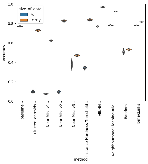
Additional to all introduced methods, we also consider a random sampling of the majority classes. The graphic above shows a first overview of all undersampling methods under accuracy for the undersampled dataset (“Partly”) and the “Full” dataset. Due to the wide range, the graphic does not give a good overview. Hence we consider the results as follows as scatter plots where we consider the mean values of the results.

We observe that working with the reduced dataset may bring better results than the baseline, which is 77% of the total dataset. As the best methods, TomekLinks, Neighbourhood Cleaning Rule, and All kNN consider still imbalanced datasets, we need to look at precision and recall for each call separately.
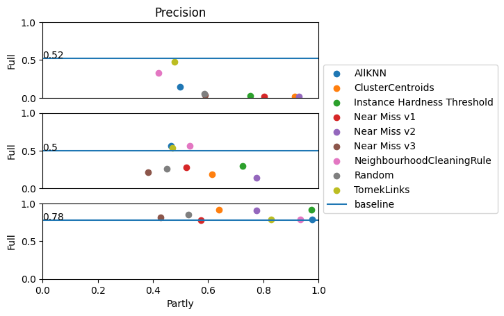
Precision gives the ratio of correct predicted classes of a specific class, and all predicted values, true positive and false negative. Hence, if the class ‘fatal’ has a prediction of 0.52, then when the model predicts this class, there is a 52% chance that this is correct. We clearly see that under-sampling improves the precision of the majority class when considering the full dataset, while the minority class gets worse results on the full dataset. Of course, we observe that considering the reduced dataset, the minority class also has good precision.
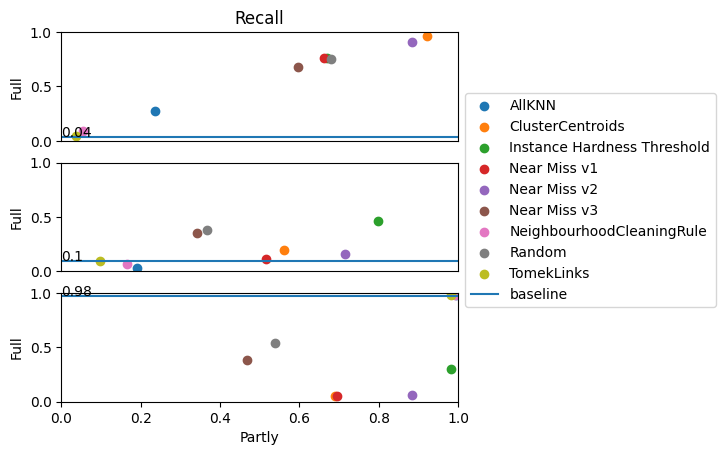
Recall gives the ratio of correct predicted classes of a specific class and all values of this class, true positive and false positive. Hence, if the class ‘serious’ has a recall of 0.1, then 10% of this class is predicted correctly. Precision and recall are like two ends of a scale: if I want a good recall, which means no false positives, then the precision decreases as the number of false negatives rises. Hence we see the same effect as at precision: the minority class improves its recall. Cluster Centroids is the best method for this approach. Class ‘Serious’ does not have good results; we see that no method gives good improvements for this class.

Recall can also be considered as a geometric mean score, where the geometric mean of the series of all recalls is considered. That means here the 3-root of the product of all recalls. This shows that all methods improve the results, but TomekLinks, Neighbourhood Cleaning Rule, and All kNN do not improve strongly enough. Random undersampling brings surprisingly good improvements, also, at Recall Graph, this belongs always to the best methods.

We also consider the macro averaged mean absolute error. Here absolute error is computed for each class separately and then averaged. The best value is 0. Also, here, random gives the best performance for the full dataset. Instance Hardness Threshold also gives good results.
Conclusion
The main idea of this study is to ask for the imbalanced dataset; how can I reduce the data such that a training method can achieve good results on the total dataset? We have different views on the results of this study. First of all, no sampling method improved performances for all classes. This holds at least for our considered dataset. Hence, we have to specify the requirements for our classifier. This is done by considering precision and recall for each class separately.
Precision can only be improved in the majority class. That means we have no false negatives but tolerate false positives. If we want to predict class ‘Slight’, then we can improve performance in the sense that predicting ‘Slight’ won’t have any misclassified samples from the classes ‘Fatal’ or ‘Serious’. However, predicting the minority classes might not be correct as there is a huge probability that the true class is ‘Slight’. If you want to be sure that when your majority class is always predicted correctly, then methods such as Instance Hardness Threshold, Cluster Centroids, or Near Miss Version 2 are the best options.
Recall can only be improved in the minority classes. That means we have no false positives but tolerate false negatives. If we want to predict a different class than ‘Fatal’, then we can improve performance in the sense that no misclassification is done. For example, predicting ‘Slight’ won’t have any misclassifications where the true class is ‘Fatal’.
Most methods bring poor performance for recall on class ‘Slight’, but for TomekLinks, Neighbourhood Cleaning Rule, and All kNN the performance remain as excellent as by trained with full dataset. This is caused as no real balancing being done.
We can not observe an excellent improvement for class ‘Seroius’.
The metrics ‘geometric mean score’ and ‘macro averaged mean absolute error’ give overall insights into the improvement of the classifier. Random undersampling is the best method for a full dataset, which improves classification. This is an interesting fact that research goes back to the 70s and is also done in more recent years. However, a better overall method than random sampling could not be found.
We will continue the search for methods solving tackling imbalanced datasets by considering oversampling methods.
References:
[01] Road Safety Data — data.gov.uk, Contains public sector information licensed under the Open Government Licence v3.0.
[02] imbalanced-learn 0.3.0.dev0 documentation (glemaitre.github.io)
[03] Violin plots explained. Learn how to use violin plots and what… U+007C by Eryk Lewinson U+007C Towards Data Science
[04] Zhang, Mani, “kNN Approach to Unbalanced Data Distributions: A Case Study involving Information Extraction”, ICML 2003
[05] Smith, Martinez, Giraud-Carrier, “An instance level analysis of data complexity”, Mach Learn 95:225–256, 2014
[06] Wilson, “Asymptotic Properties of Nearest Neighbor Rules Using Edited Data”, IEEE Transactions on Systems, Man, and Cybernetics, 1972
[07] Tomek, “An Experiment with the Edited Nearest-Neighbor Rule”, IEEE Transactions on Systems, Man, and Cybernetics, 1976
[08] Laurikkala, “Improving Identification of Difficult Small Classes by Balancing Class Distribution”, Lecture Notes in Computer Science, 2001
[09] UMAP: Uniform Manifold Approximation and Projection for Dimension Reduction — umap 0.5 documentation
[10] How Exactly UMAP Works. And why exactly it is better than tSNE U+007C by Nikolay Oskolkov U+007C Towards Data Science (medium.com)
Join thousands of data leaders on the AI newsletter. Join over 80,000 subscribers and keep up to date with the latest developments in AI. From research to projects and ideas. If you are building an AI startup, an AI-related product, or a service, we invite you to consider becoming a sponsor.
Published via Towards AI
Related posts


Popular posts

 for 2021")


Updates

Recent Posts


