Solving the Vanishing Gradient Problem with Self-Normalizing Neural Networks using Keras

Last Updated on October 23, 2020 by Editorial Team

Author(s): Jonathan Quijas

Machine Learning

How to Improve Convergence and Performance of Deep Feed-Forward Neural Networks via a Simple Model Configuration

Problem Statement

Training deep neural networks can be a challenging task, especially for very deep models. A major part of this difficulty is due to the instability of the gradients computed via backpropagation. In this post, we will learn how to create a self-normalizing deep feed-forward neural network using Keras. This will solve the gradient instability issue, speeding up training convergence, and improving model performance.

Disclaimer: This article is a brief summary with focus on implementation. Please read the cited papers for full details and mathematical justification (link in sources section).

Background

In their 2010 landmark paper, Xavier Glorot and Yoshua Bengio provided invaluable insights concerning the difficulty of training deep neural networks.

It turns out the then-popular choice of activation function and weight initialization technique were directly contributing to what is known as the Vanishing/Exploding Gradient Problem.

In succinct terms, this is when the gradients start shrinking or increasing so much that they make training impossible.

Saturating Activation Functions

Before the wide adoption of the now ubiquitous ReLU function and its variants, sigmoid functions (S-shaped) were the most popular choice of the activation function. One such example of a sigmoid activation is the logistic function:

One major disadvantage of sigmoid functions is that they saturate. In the case of the logistic function, the outputs saturate to either 0 or 1 for negative and positive inputs respectively. This leads to smaller and smaller gradients (very close to 0) as the magnitude of the inputs increases.

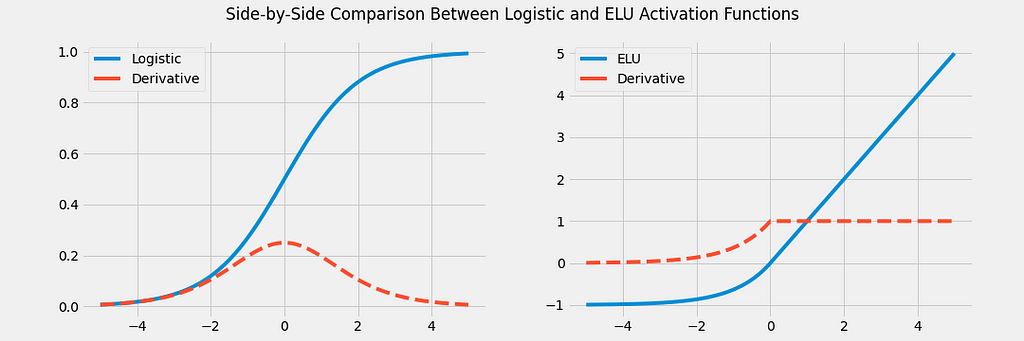
Since the ReLU and its variants do not saturate, they alleviate this vanishing gradient phenomenon. Improved variants of the ReLU such as the ELU function (shown above) have smooth derivatives all across:

• For any positive input, the derivative will always be 1
• For small negative numbers, the derivative will not be close to zero
• Smooth derivative all across

NOTE: It is therefore beneficial to have inputs with an expected value of 0, as well as a small variance. This would help maintain strong gradients across the network.

Poor Choice of Weight Initialization

Another important insight found in the paper was the effect of weight initialization using a normal distribution with 0 mean and standard deviation of 1, a widely-popular choice prior to the authors’ findings.

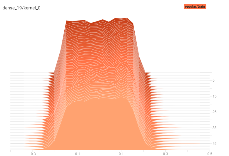
The authors showed that the particular combination of a sigmoid activation and weight initialization (a normal distribution with 0 mean and standard deviation of 1) makes the outputs have a larger variance than the inputs. This effect is compounded across the network, making the input of deeper layers have a much larger magnitude relative to the input of more shallow (earlier) layers. This phenomenon was later named Internal Covariate Shift in a 2015 landmark paper by Sergey Ioffe and Christian Szegedy.

As we saw above, this translates into smaller and smaller gradients when using sigmoid activations.

The problem is further accentuated with the logistic function, since it has an expected value of 0.5, rather than 0. The hyperbolic tangent sigmoid function has an expected value of 0, and thus behaves better in practice (but also saturates).

The authors argued that in order for the gradients to be stable during training, the inputs and outputs of all layers must preserve more or less the same variance across the entire network. This would prevent the signal from dying or exploding when propagating in a forward pass, as well as gradients vanishing or exploding during backpropagation.

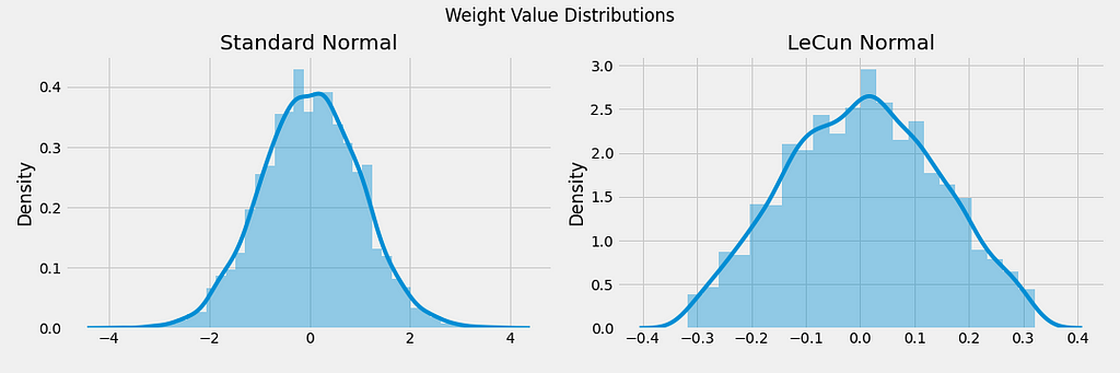
To achieve this, they proposed a weight initialization technique, named Glorot (or Xavier) initialization after the paper’s first author. It turns out that with a slight modification of the Glorot technique, we get LeCun initialization, named after Yann LeCun.

Yann LeCun proposed his LeCun initialization in the 1990’s, with references found in the Springer publication Neural Networks: Tricks of the Trade (1998).

Self-Normalizing Feed Forward Neural Networks (SNNs)

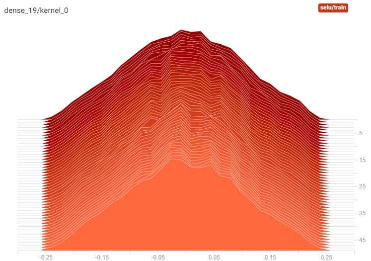
In 2017, Günter Klambauer et al. introduced self-normalizing neural networks (SNNs). By ensuring some conditions are met, these networks are able to preserve outputs close to 0 mean and standard deviation of 1 across all layers. This means SNNs do not suffer from the vanishing/exploding gradient problem and thus converge much faster than networks without this self-normalizing property. According to the authors, SNNs significantly outperformed the other variants (without self-normalization) in all learning tasks reported in the paper. Below is a more detailed description of the conditions needed to create an SNN.

Architecture and Layers

An SNN must be a sequential model comprised only of fully-connected layers.

NOTE: Certain types of networks are more adequate than others depending on the task. For example, convolutional neural networks are commonly used in computer vision tasks, primarily due to their parameter efficiency. Make sure a fully-connected layer is adequate for your task. If this is the case, then consider using a SNN. Otherwise, Batch Normalization is an excellent way to ensure proper normalization across the network.

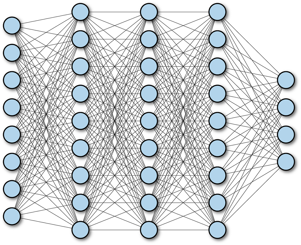
A sequential model in this case refers to one where layers are in a strict sequential order. In other words, for each hidden layer l, the only inputs layer l receives are strictly the outputs of layer l-1. In the case of the first hidden layer, it only receives the input features. In Keras, this type of model is in fact referred to as a Sequential model.

A fully connected layer is one where each unit in the layer has a connection to every single input. In Keras, this type of layer is referred to as a Dense layer.

Input Standardization

The input features must be standardized. This means the training data should have 0 mean and standard deviation of 1 across all features.

Weight Initialization

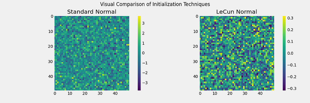
All layers in an SNN must be initialized using the LeCun Normal initialization. As we saw earlier, this will ensure the range of weight values lies closer to 0.

The SELU Activation Function

The authors introduced the Scaled ELU (SELU) function as the activation function for SNNs. As long as the previous conditions are met, the SELU provides a guarantee of self-normalization.

Keras Implementation

The following example shows how to define an SNN for a 10-class classification task:

def get_model(num_hidden_layers=20, input_shape=None, hidden_layer_size=100):

   model = keras.models.Sequential()

   model.add(keras.layers.Flatten(input_shape=input_shape))

   for layer in range(num_hidden_layers):

      model.add(keras.layers.Dense(hidden_layer_size,    activation='selu', kernel_initializer='lecun_normal'))

      model.add(keras.layers.Dense(10, activation='softmax'))

   return model

Experimental Results

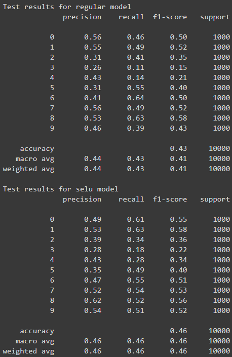
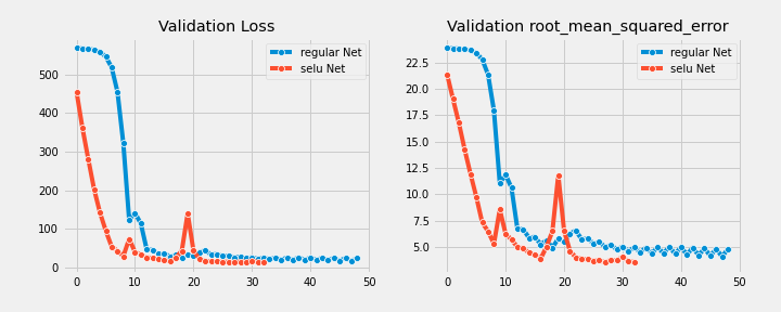
Below is the comparison between a regular feed-forward neural network and an SNN on three different tasks:

• Image classification (Fashion MNIST, CIFAR10)
• Regression (Boston housing dataset)

Both networks shared the following configuration:

• 20 hidden layers
• 100 units per hidden layer
• Nadam optimizer
• Learning rate of 7e-4
• 50 epochs

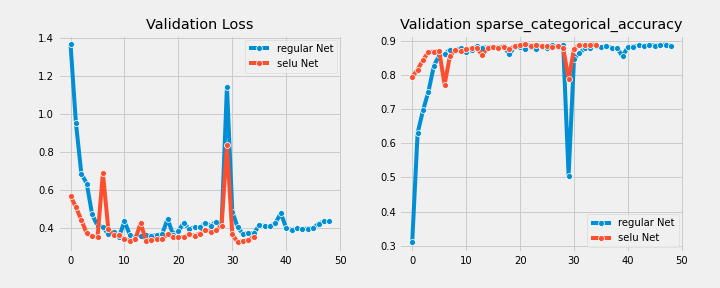
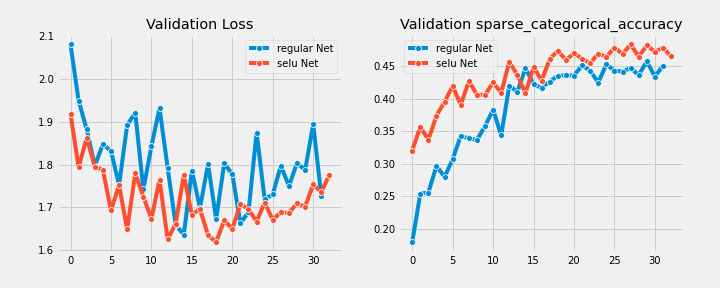
For both models, the learning curves stop at the epoch where the best performance metric was achieved

Fashion MNIST

CIFAR10

Boston Housing

Conclusion

By ensuring our feed-forward neural network configuration meets a set of conditions, we can get it to automatically normalize. The required conditions are:

• The model must be a sequence of fully-connected layers
• Weights are initialized with the LeCun normal initialization technique
• The model uses the SELU activation function
• Inputs are standardized

This almost always will lead to improved performance and convergence compared to models without self-normalization. If your task requires a regular feed-forward neural network, consider using the SNN variant. Otherwise, Batch Normalization is an excellent (but more time and compute costly) normalization strategy.

Sources

• Glorot, Xavier, and Yoshua Bengio. “Understanding the difficulty of training deep feedforward neural networks.” Proceedings of the thirteenth international conference on artificial intelligence and statistics. 2010.
• Ioffe, Sergey, and Christian Szegedy. “Batch normalization: Accelerating deep network training by reducing internal covariate shift.” arXiv preprint arXiv:1502.03167 (2015).
• Klambauer, Günter, et al. “Self-normalizing neural networks.” Advances in neural information processing systems. 2017.
• Montavon, Grégoire, G. Orr, and Klaus-Robert Müller. “Neural networks-tricks of the trade second edition.” Springer, DOI 10 (2012): 978–3.
• Hands-on Machine Learning with Scikit-Learn, Keras and TensorFlow
• https://en.wikipedia.org/wiki/Logistic_function
• https://en.wikipedia.org/wiki/Vanishing_gradient_problem
• https://en.wikipedia.org/wiki/Backpropagation
• https://en.wikipedia.org/wiki/Normal_distribution

---

Solving the Vanishing Gradient Problem with Self-Normalizing Neural Networks using Keras was originally published in Towards AI on Medium, where people are continuing the conversation by highlighting and responding to this story.

Published via Towards AI