


Predicting Heart Failure Survival with Machine Learning Models — Part II
Last Updated on July 19, 2023 by Editorial Team
Author(s): Anirudh Chandra
Originally published on Towards AI.
The second part of the step-by-step walk-through to analyze and predict the survival of heart failure patients.
Preface
In the previous post, we looked at the heart failure dataset of 299 patients, which included several lifestyle and clinical features. That post was dedicated to an exploratory data analysis while this post is geared towards building prediction models.
Motivation
The motivating question is— ‘What are the chances of survival of a heart failure patient?’. Through this walk-through, I try to answer this question while also giving a few insights on dealing with imbalanced datasets.
The code for this project can be found on my GitHub repository.
Quick Recap
In the previous post, we saw that —
- Age and serum creatinine had a slightly positive correlation, while serum sodium and serum creatinine had a slightly negative correlation.
- Most of the patients who died had no co-morbidities or at the most suffered from anemia or diabetes.
- The ejection fraction seemed to be lower in deceased patients than in patients who survived.
- The creatinine phosphokinase level seemed to be higher in deceased patients than in patients who survived.
(Check out the previous post to get a primer on the terms used)
Outline
- Dealing with Class Imbalance
- Choosing a Machine Learning model
- Measures of Performance
- Data Preparation
- Stratified k-fold Cross-Validation
- Model Building
- Consolidating Results
1. Dealing with Class Imbalance
Before putting on our hard hats, let’s have a quick look at the balance of target classes. We look at the proportion of deceased and survivors in the original data set.
print('% of heart failure patients who died = {}'.format(df.death.value_counts(normalize=True)[1]))
print('% of heart failure patients who survived = {}'.format(df.death.value_counts(normalize=True)[0]))% of heart failure patients who died = 0.3210702341137124
% of heart failure patients who survived = 0.6789297658862876
We see that 32% of the patients died, while 68% survived. This is clearly an imbalanced dataset!. In which case, whatever model we choose has to account for this imbalance.
Dealing with imbalanced data is pretty common in the real-world and these articles by
German Lahera and on DataCamp are good places to learn about them.
A technical overview of solving this problem goes like this — You can assign a penalty to the misclassification of the minority class (The one with the lesser proportion) and by doing so, allow the algorithm to learn this penalization. The other approach is to use a sampling technique: Either down-sampling the majority class or oversampling the minority class, or both [1].
In our exercise, we will try to deal with this imbalance by —
- Using a stratified k-fold cross-validation technique to make sure our model’s aggregate metrics are not too optimistic (meaning: too good to be true!) and reflect the inherent imbalance in the training and testing data;
- Using a penalized model (instead of a sampling technique like SMOTE) with a simple weighting scheme that is the inverse of a class frequency.
By following these steps, we will observe the effect of imbalance on the model prediction and try to derive some insights!
2. Choosing a machine learning model
For this post, we will consider the problem at hand to be a supervised classification problem and look at two basic linear models—
- Logistic Regression (LogReg)
- Support Vector Machines (SVM)
We are sticking to these workhorses because they have some neat tricks to deal with imbalanced target labels and are easy to understand. Feel free to try other algorithms such as Random Forests, Decision Trees, Neural Networks, etc., among supervised models and k-nearest neighbors, DBSCAN, etc., among unsupervised models.
3. Measures of performance
Any prediction model must be assessed on its performance by means of certain prediction metrics. Before we do that let us define our types of cases —
- True Positives (TP): When the model predicts death and the patient died;
- True Negatives (TN): When the model predicts survival and the patient survived;
- False Positives (FP): When the model predicts death but the patient survived;
- False Negatives (FN): When the model predicts survival but the patient died.
Using these case types, we define the following 5 prediction metrics —
- Recall: This is also known as True Positive Rate or Sensitivity of the model to true positives. It is computed as TP/(TP + FN).
- Precision: This is a measure of how precise the true positives predicted by the model are. It is computed as TP/(TP+FP).
- Accuracy: This is an aggregate measure of the overall performance of the model and is computed as (TP+TN)/(TP+TN+FP+FN).
- Balanced Accuracy: This is an aggregate measure of the model’s ability to classify each class. It is the average of the sensitivity (TPR) and specificity (TNR) and is given as (TPR + TNR)/2.
- ROC AUC: This is the area under the Receiver Operating Characteristic Curve (ROC) curve that is generated by the true positive rate and false-positive rate for different prediction thresholds. For a random predictor, this value is 0.5 and our model must be better than that.
Having defined these metrics, it is important to outline the kind of performance we expect our model to have. We expect the prediction model to have —
- High Recall— The model must be able to predict as many deaths as possible;
- High Precision— The deaths predicted by the model must be precise, ie, match with the observed deaths, as often as possible;
- High Balanced Accuracy — The model must be able to predict deaths and survivals equally well, ie, the model must be sensitivity to as many deaths as possible and at the same time, be specific in its death and survival predictions;
- High Accuracy — The model must have had a high overall accuracy;
- High ROC AUC — The model’s overall area under the curve must be greater than any random predictor’s value of 0.5.
4. Data Preparation
Scaling the data
Our primary data preparation would be a feature scaling. We do this with numerical features because they are measured on different scales. We use the StandardScaler() method in sklearn.preprocessing and scale the values so that they have a mean 0 and variance 1.
cat_feat = df[['sex', 'smk', 'dia', 'hbp', 'anm']]
num_feat = df[['age', 'plt', 'ejf', 'cpk', 'scr', 'sna']]predictors = pd.concat([cat_feat, num_feat],axis=1)
target = df['death']from sklearn.preprocessing import StandardScalerscaler = StandardScaler()
scaled_feat = pd.DataFrame(scaler.fit_transform(num_feat.values),
 columns = num_feat.columns)
scaled_predictors = pd.concat([cat_feat, scaled_feat], axis=1)
(We drop the time feature in the current analysis)
5. Stratified k-fold cross-validation
A quick primer
Now, these models that we chose have a certain degree of stochasticity to them, especially when it comes to solving for coefficients. This means that our results would change a little every time we run the model. To make sure that we minimize this randomness, prevent under-fitting or over-fitting, we run the model multiple times and calculate the average of the metric of our choice.
k-fold cross-validation is a well-known method of doing this iterative validation, especially with small datasets that may not be perfectly representative of the population under study. The dataset is split into k subsets and the model is trained on the first k-1 subsets and tested on the last kth subset. This process is repeated k times and the average of the performance measures is calculated [2].
Stratified k-fold cross validation comes to the rescue when the target labels are imbalanced. Since the usual k-fold cross-validation on imbalanced targets may cause a few training sets to have only one target label to train on, stratification is carried out. In other words, the earlier process is repeated, but this time, making sure that the proportion of target labels are maintained in each training set [3][4].
We use StratifiedKFold and cross_validatefrom sklearn.model_selection to carry out 10-fold cross-validation, after which we tally the listed metrics.
(I have found
Jason Brownlee’s machinelearningmastery.com to be a supremely useful resource to learn more on this)
6. Model Building
Logistic Regression
Logistic Regression is a class of linear regression models that is typically suited for predicting binary outcomes.It gives out a non-linear output for a linear input. At its heart is the logistic function (a sigmoid function) and the class probabilities are assigned based on this function after suitable update of regression coefficients.
To emphasis the effect of bias creeping in from the imbalanced target classes, we run the logistic regression model with and without penalization. The penalization can simply be enabled by class_weight=’balanced’ while instantiating the Logistic Regression model.
#Stratified 8 fold cross validation
strat_kfold = StratifiedKFold(n_splits=10, shuffle=True)#Instantiating the logistic regressor
logreg_clf = LogisticRegression() #To enable penalization, assign 'balanced' to the class_weight parameterx = scaled_predictors.values
y = target.values#Running the model and tallying results of stratified 10-fold cross validation
result = cross_validate(logreg_clf, x, y, cv=strat_kfold, scoring=['accuracy','balanced_accuracy', 'precision', 'recall', 'roc_auc'])
We take a look at the prediction results from the non-penalized and penalized logistic regression model.
pd.concat([pd.DataFrame(result1).mean(),
 pd.DataFrame(result2).mean()],axis=1).rename(columns={0:'Non-Penalized LogReg',1:'Penalized LogReg'})

Some interesting observations —
- The overall accuracy of the two models is pretty much the same at ~72%, which is reasonably good.
- But when we look at the balanced accuracy we see a major difference. The penalized LogReg was sensitive to both the classes (71%), while the non-penalized LogReg was less sensitive (66%).
- The precision is on the lower side for the penalized LogReg (54%) than the non-penalized LogReg (67%), with the values not nearly high enough.
- The greatest jump insensitivity or recall to deaths is seen in the penalized LogReg (72%) over the non-penalized LogReg (44%).
- The ROC AUC at 0.76–0.77 is still better than a random classifier.
Support Vector Classifier
SVCs are non-parametric classifiers that use hyperplanes in feature space to try and separate the data points into classes that are close to one another. Watch this video by StatQuest on Youtube for a clear explanation!
From the EDA in the previous post, we saw that quite a few data points classified as deceased are found in the periphery of the scatter plots. We can perhaps presume that a linear kernel would not be able to separate these data points adequately and instead go for a radial basis function kernel.
We instantiate a penalized as well as a non-penalized SVC in the same manner as before and take stock of the bias that creeps in while predicting imbalanced classes.
#Stratified 10 fold cross validation
strat_kfold = StratifiedKFold(n_splits=10, shuffle=True)#Instantiating the SVC
svc_clf = SVC(kernel='rbf')
x = scaled_predictors.values
y = target.values#Running the model and tallying results of stratified 10-fold cross validation
result3 = cross_validate(svc_clf, x, y, cv=strat_kfold, scoring=['accuracy','balanced_accuracy','precision','recall','roc_auc'])
We compare the prediction results from the two variations of the SVC model.
pd.concat([pd.DataFrame(result3).mean(),
 pd.DataFrame(result4).mean()],axis=1).rename(columns={0:'Non-Penalized SVC',1:'Penalized SVC'})
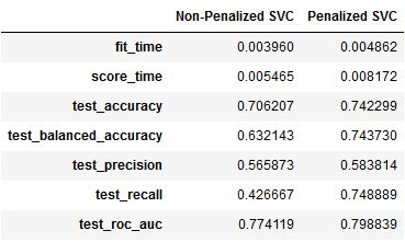
Some interesting observations —
- The overall accuracy (74%) and balanced accuracy (74%) of the penalized SVC are greater than the non-penalized SVC.
- The precision, unlike the LogReg model, is on the lower side for both the variations of the SVC.
- The greatest jump in sensitivity or recall to deaths is seen in the penalized SVC (75%) over the non-penalized SVC (43%).
- The ROC AUC at 0.77–0.80 is still better than a random classifier.
7. Consolidating Results
At the end of this exercise, it is important that we take stock of the results obtained so far and make some sense of the insights gained along the way.
- In this dataset of 299 heart failure patients, 68% survived while 32% did not survive;
- 5 lifestyle features and 5 clinical features characterize this dataset and were used as potential predictors for survival;
- Most of those who died had no co-morbidities, had lower ejection fraction and higher creatinine phosphokinase levels than the survivors;
- When traditional linear classification models such as Logistic Regression and Support Vector Machines are used to predict survival, the imbalance in the dataset affects the performance;
- 10-fold cross-validation and an inverse frequency penalization scheme improves the prediction performance of these models;
- The penalized SVC is marginally better than the penalized LogReg for predicting deaths for this dataset;
- The two models have good ability (>70%) to differentiate between those likely to survive and those likely to die, using the 10 features provided.
- Given a heart failure patient’s medical history (5 life style and 5 clinical histories), these two models have at least 70% accuracy in predicting the patients' survival.
Some interesting aspects that can lift the merit of this project are — PCA and CATPCA to eliminate highly correlated features, hyper-parameter testing, trying unsupervised machine learning models, etc.
That’s the end of this project and I hope you found the two posts useful. Feedback is most welcome!
Ciao!
References
[1] https://statistics.berkeley.edu/sites/default/files/tech-reports/666.pdf
[2]https://machinelearningmastery.com/k-fold-cross-validation/
[3]https://scikit-learn.org/stable/modules/generated/sklearn.model_selection.StratifiedKFold.html
[4]https://machinelearningmastery.com/k-fold-cross-validation/
Join thousands of data leaders on the AI newsletter. Join over 80,000 subscribers and keep up to date with the latest developments in AI. From research to projects and ideas. If you are building an AI startup, an AI-related product, or a service, we invite you to consider becoming a sponsor.
Published via Towards AI
Related posts


Popular posts

 for 2021")


Updates

Recent Posts


