
 Logo:
Logo:  Areas Served:
Perfect Answer to Deep Learning Interview Question — Why Not Quadratic Cost Function?
Last Updated on June 11, 2024 by Editorial Team
Author(s): Varun Nakra
Originally published on Towards AI.
One of the most common question asked during deep learning knowledge interviews is — “Why can’t we use a quadratic cost function to train a Neural Network?”. We will delve deep into the answer for that. There will be a lot of Math involved but nothing crazy! and I will keep things simple yet precise.
Let’s start with contemplating on the general architecture of a Neural network

We have a series of inputs forming an “input layer”, a series of neurons in the “hidden layer” and one neuron forming an “output layer” for a binary classification problem. For the purposes of this question, we will assume that we are dealing with a binary classifier, so we have just one output value coming out of the network.
Now look at the following figure where we’ve highlighted the input layer in green and output neuron in red and one neuron of the hidden layer in orange. From all greens to the orange, we see that all inputs are connected to the orange neuron. In other words, the “activation” of the orange neuron happens using the “aggregation” of all the green neurons in the input layer. This process is replicated over all neurons over all layers until we reach the final red output neuron.

What if we replace the orange neuron with the red neuron, i.e., we remove the hidden layer and connect the red neuron with the green neurons directly?

We will get the following

For the purposes of this question, we will assume the aforementioned ‘simplistic architecture’ and the result can be generalized to the complete architecture as well. Now let’s introduce some Math step-by-step.

What we see above is the basic “weight update” equation for a Neural network. I have removed the extra hyperparameters such as the learning factor and the sub-sampling (min-batch), etc. w_k is the vector of weights and the weights are the ‘parameters’ of our Neural network model. w_k comprises individual weights gathered in a column vector. These weights are associated with the inputs to the model (that is the green neurons in our architecture). We have a cost function C_i where i = 1 to n are the number of data instances in our sample. The cost function C is the “error” between the actual output y and the output from the neural network (red neuron). It is evident that each data instance will produce a predicted output as against an actual output, therefore, there will be a cost or error for every data instance. The objective of the model is to minimize this cost function on an average over the entire dataset. And as we know the minimization step involves taking a derivative with respect to the model parameters (weights), we do that using the partial derivative with respect to the vector w_k. All this means is that the cost C will be an expression/aggregation of weights w_1 to w_q and we will differentiate with respect to each weight w and collect that in a vector. This is called as the negative “gradient vector”. And it is used to update the weight vector from the k-th iteration to the (k+1)th iteration. The methodology is Stochastic Gradient descent but we will leave that out for this article. In a nutshell, the neural network learns by an update to the weights via the negative gradient vector averaged over all the samples and calculated for w_k. This helps us move to the minimization of the cost function and helps the network to learn and improve its accuracy. It is obvious that if the updates to the weights are not happening because the negative gradient is moving towards zero, the learning has stopped. This doesn’t necessarily imply that we have reached the minimum! Because our cost function is highly complicated and we need to find a minimum in a multi-dimensional space. Therefore, there could be many local minima where the gradient is zero and the network stops learning. Anyway, we don’t have to worry about that for this problem. Let’s look at the following expression

This expression defines z_i as a weighted sum of the inputs x_ji. Note that these inputs are the green neurons in our architecture. As we have no hidden layer, we combine the inputs x_ji and the weights w_j and add a bias term to get z_i which is what is represented by the connecting arrows from the green neurons to the red neuron in our architecture. Since, we have q inputs, we have x_j and w_j where j = 1 to q

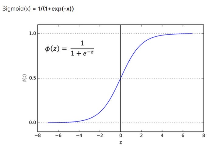
But, we don’t pass z_i to the red neuron. We apply an “activation function” to it. This activation function can be different for different neural networks. For the purposes of this problem, we assume the activation function is “Sigmoid” or “logistic”. I will assume here that the reader is aware of this function and move on further.
Next comes our main problem statement — How do we define the Cost function C? It is well known that for binary classification, the cost function is “Cross entropy” but the question here is why can’t it be “Quadratic”. Let’s define the expressions of both the cost functions
Quadratic cost function –

Cross Entropy cost function –

Whilst the quadratic cost function is straightforward (think least squares minimization between the actual output y_i and the predicted output a_i), we can offer some explanation for the cross-entropy cost function. This is akin to negative log-likelihood in our regression models. Note that there is a negative sign outside the brackets, which is used to keep the cost positive (because a_i will be between 0 and 1 — an output of sigmoid; therefore, the term inside the brackets will be always negative). Also note that when a_i gets really close to y_i, the cost gets really close to zero. This is because, when y_i = 1 and a_i ~ 1, ln(a_i) will be approximately 0. Similarly, when y_i= 0 and a_i ~ 0, ln(1-a_i) will be approximately 0. Thus, this function keeps the cost positive and minimal when the model is predicting well. However, the same can be said about the quadratic cost function as well. But, we don’t use it. Why? Here comes the explanation
We go back to the basic weight update equation we saw earlier and input the quadratic cost function to it. We get the following

Now to keep things simple, we will consider only one data point, that is i=1 and n=1. And we differentiate partially with respect to each weight w_j. We get the following

Recall that since i = 1, we have

Substituting the value of z, we get

That is, our gradient vector, which is responsible for updating the weights of the network, will have a derivative of the sigmoid function when we use a quadratic cost function. Now, let’s look at the behavior of the derivative of the sigmoid function
From the above plot, it is clear that the derivative, representing the slope of the sigmoid function, approaches 0 as soon as the input z becomes large! What does this mean? This means that the gradient vector will be zero when the activation input z is large. Therefore, the network will stop learning as the weights won’t get updated. Recall that this does not mean we have reached a minimum. This means, we are stuck at an undesirable point and in the function space, which could be far from the minimum value. This is known as “learning slow down”. However, this does NOT occur with a cross-entropy cost function. We perform the same substitution using the cross-entropy cost function and get the following:

It is interesting to note that the term

occurs in the gradient for quadratic cost as well. However, there is a trick which we will use to simplify it. The gradient of the sigmoid function can be expressed as follows

We substitute that into our original expression and get the following

That is our gradient vector, which is responsible for updating the weights of the network, does not have a derivative of the sigmoid function when we use a cross-entropy cost function. Hence, there is no slowdown of learning with this cost function.
We juxtapose the gradients again for a better look.


This answers our original question — we don’t use the quadratic cost function because it leads to a slowdown of learning. Note that the above analysis was done only on the output layer (of one neuron), however, it is can be generalized for a general neural network as well!
Join thousands of data leaders on the AI newsletter. Join over 80,000 subscribers and keep up to date with the latest developments in AI. From research to projects and ideas. If you are building an AI startup, an AI-related product, or a service, we invite you to consider becoming a sponsor.
Published via Towards AI
Related posts
Popular posts

 for 2021")


Updates

Recent Posts
