Neural Network from Scratch

Author(s): Abhishek Chaudhary

Originally published on Towards AI.

Many of us have a functional understanding of neural networks and how they work. I’ve even studied this particular term multiple times, and every time, I convince myself that I know what I’m talking about. The human brain is funny that way; it takes the path of least resistance and convinces us that we know something when we don’t. Though I’ve used neural networks multiple times for tasks ranging from binary classification to natural language processing, I’ve never really implemented them from scratch, and if you’re like me, then your understanding of neural networks ends at Y = WX + b.

In this article, I’ll implement a neural network from scratch, going over different concepts like derivatives, gradient descent, and backward propagation of gradients. I would also like to mention that this article is inspired by Anderj Karapthy’s brilliant lecture series on YouTube, and I will be making use of some of the code mentioned in that video.

This article also has a corresponding Jupyter notebook with all of the code that’s covered below.

Introduction

Feel free to skip to the next section, as the introduction section covers the theory of neural networks and not the implementation.

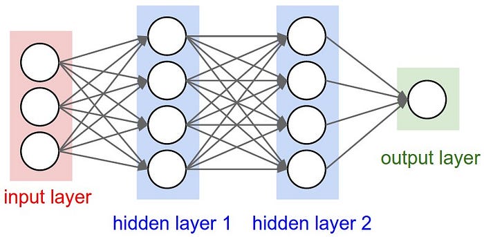
Neural networks are a type of machine model inspired by the structure of the human brain. Similar to our brain, Neural networks are made up of Neurons that work together to accomplish a whole variety of tasks. The diagram below shows the architecture of a neuron:

Where :

• output: This is the final value or activation of the neuron.
• activation_function: This is a mathematical function that determines whether the neuron should fire or not based on its input.
• weighted_sum: It is the sum of the products of the input values and their corresponding weights.
• bias: A bias term is added to the weighted sum to provide the neuron with some flexibility in its activation.

The weighted sum is calculated as follows: weighted_sum = (w1 * x1) + (w2 * x2) + ... + (wn * xn) Where:

• w1, w2, ..., wn: These are the weights associated with each input.
• x1, x2, ..., xn: These are the input values.

The activation function can be any non-linear function, such as the sigmoid, ReLU (Rectified Linear Unit), or softmax function, depending on the type of neuron and the task at hand.

The role of the activation function is to introduce non-linearity into the neuron’s output, allowing it to learn complex patterns and relationships in the data.

In summary, a single neuron in a neural network takes input values, applies weights to them, sums them up with a bias term, and then passes the result through an activation function to produce an output. This output is then used as input for subsequent layers or neurons in the neural network, enabling the network to learn and make predictions for various tasks.

Now, with all the theory out of the way, let’s implement a neuron. Starting with derivatives.

Getting rid of the imports early on in the process

import math
import numpy as np
import matplotlib.pyplot as plt
%matplotlib inlinep

Derivatives

Before moving to neuron and neural networks, let’s briefly go over the functions and their derivatives. As all of us have learned in school, A derivative of a function with respect to a variable shows the rate of change of the function with respect to that variable.

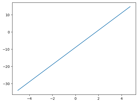
What does this mean for a function, say f(x) = 5x - 9?

f'(x)=5 i.e., the function f(x) increases by a factor of 5 for 1 unit change in x. We can also calculate this value by nudging x by an infinitesimal value h and observe how f(x) changes. i.e

f(x) = 5x - 9
f(x+h) = 5(x+h) - 9
f`(x) = (f(x+h) - f(x))/(x+h - x) = 5 --> 

This is also referred to as rise-over-run

Multivariate functions

For a multivariate functions such as d = a*b + c, the rate of change is different for different variables.

def f(x):
 return 5*x - 9

xs = np.arange(-5,5,0.25)
ys = f(xs)
plt.plot(xs, ys)

[<matplotlib.lines.Line2D at 0x130c99290>]

Implementation of a Value in Neural Network

Pytorch makes use of Tensors for computation, to replicate the functionality, we'll write our own implementation Value

class Value:
 def __init__(self, data, label=''):
 self.data = data
 self.label = label
 self.grad = 0.0 # We'll go over this field in detail later on
 def __repr__(self):
 return f"Value=(data={self.data}, label={self.label})"

'''
Let's make use of a multi-variate equation and write it using the Value class defined above
a = 2.0
b = -3.0
c = 10.0
e = a * b
d = e + c
f = -2.0
l = d * f
'''
a = Value(2.0, label='a')
b = Value(-3.0, label='b')
c = Value(10.0, label='c')
e = a*b

---------------------------------------------------------------------------

TypeError Traceback (most recent call last)

Cell In[92], line 14
 12 b = Value(-3.0, label='b')
 13 c = Value(10.0, label='c')
---> 14 e = a*b


TypeError: unsupported operand type(s) for *: 'Value' and 'Value'

The error above shows that * isn’t defined for the Value type. We’ll need to modify the Value type to support + and * operations.
We’ll also add an op field that shows how the Value was created. Since we are working with a neural network, we’ll need to keep track of the children of a node. So we’ll add a _prev field to the Value type

class Value:
 def __init__(self, data, _children=(), _op='', label=''):
 self.data = data
 self.label = label
 self._op = _op
 self._prev = set(_children)
 self.grad = 0
 
 def __repr__(self):
 return f"Value=(data={self.data}, label={self.label})"
 
 def __add__(self, other):
 out = Value(self.data + other.data, (self, other), '+')
 return out

 def __mul__(self, other):
 out = Value(self.data * other.data, (self, other), '*')
 return out

a = Value(2.0, label='a')
b = Value(-3.0, label='b')
c = Value(10.0, label='c')
e = a*b; e.label = 'e'
d = e + c; d.label = 'd'
f = Value(-2.0, label='f')
L = d * f; L.label = 'L'
L

Value=(data=-8.0, label=L)

For visualizing the network, we’ll make use of graphviz. The code below is directly referenced from https://github.com/karpathy/nn-zero-to-hero/blob/master/lectures/micrograd.

from graphviz import Digraph

def trace(root):
 # builds a set of all nodes and edges in a graph
 nodes, edges = set(), set()
 def build(v):
 if v not in nodes:
 nodes.add(v)
 for child in v._prev:
 edges.add((child, v))
 build(child)
 build(root)
 return nodes, edges

def draw_dot(root):
 dot = Digraph(format='png', graph_attr={'rankdir': 'LR'}) # LR = left to right
 
 nodes, edges = trace(root)
 for n in nodes:
 uid = str(id(n))
 # for any value in the graph, create a rectangular ('record') node for it
 dot.node(name = uid, label = "{ %s U+007C data %.4f U+007C grad %.4f }" % (n.label, n.data, n.grad), shape='record')
 if n._op:
 # if this value is a result of some operation, create an op node for it
 dot.node(name = uid + n._op, label = n._op)
 # and connect this node to it
 dot.edge(uid + n._op, uid)

 for n1, n2 in edges:
 # connect n1 to the op node of n2
 dot.edge(str(id(n1)), str(id(n2)) + n2._op)

 return dot

''' 
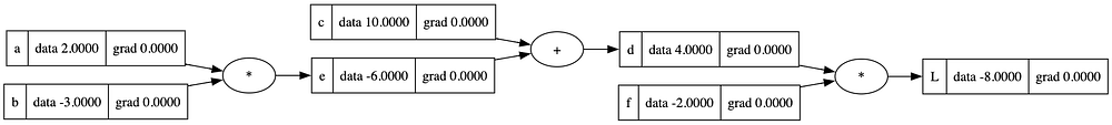
Plotting the variable L to layout the network. The _op nodes are just rendered to show the parent/child relation between nodes
'''
draw_dot(L)

Derivatives/Gradient

Manually computing gradient, moving backward from L, which is the base case with a gradient of 1.0

L.grad = 1.0 # Base case as rate of change of L wrt to L is 1
''' 
We know that L = d*f
so dL/de (gradient of L wrt to f or rate of change of L wrt to f) = d
similarly dL/dd will be f
'''

d.grad = f.data
f.grad = d.data

''' 
Since d = e + c, to find out dL/dd (Rate of change of L wrt to d) we'll make use of the chain rule i.e
dL/de = (dL/dd) * (dd/de) = (dL/dd) * 1.0
similarly dL/dc = dL/dd * 1.0
'''
e.grad = d.grad
c.grad = d.grad

''' 
e = a * b
So following the chain rule again
dL/da = (dL/de) * (de/da) = (dL/de) * b
dL/db = (dL/de) * (de/db) = (dL/de) * a
'''
a.grad = e.grad * b.data
b.grad = e.grad * a.data

''' 
Plotting the variable L to layout the network.
'''
draw_dot(L)

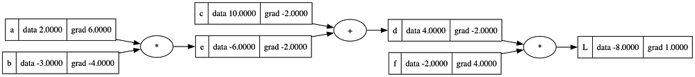
From the diagram above, we can make a simple observation that + nodes transfer gradients from child node to parent nodes, for example, the gradient of e and c are the same as that of d. Now that we have established the concepts of gradients. Let’s move towards expression representing a Neuron.

# inputs x1,x2
x1 = Value(2.0, label='x1')
x2 = Value(0.0, label='x2')

# weights w1,w2
w1 = Value(-3.0, label='w1')
w2 = Value(1.0, label='w2')

# bias of the neuron
b = Value(6, label='b')

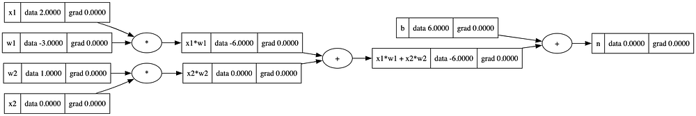
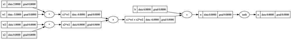
# x1*w1 + x2*w2 + b
x1w1 = x1*w1; x1w1.label = 'x1*w1'
x2w2 = x2*w2; x2w2.label = 'x2*w2'

x1w1x2w2 = x1w1 + x2w2; x1w1x2w2.label = 'x1*w1 + x2*w2'

n = x1w1x2w2 + b; n.label = 'n'

draw_dot(n)

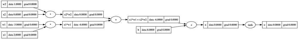
Activation function

Neurons also make use of something called an activation function. Activation functions introduce non-linearity into the neural network, allowing it to model complex relationships and learn from data. For the purpose of this article, we’ll use tanh as our activation function. The tanh function squashes the net input, but it maps it to a range between -1 and 1. It is often used in hidden layers of neural networks.

plt.plot(np.arange(-5,5,0.2), np.tanh(np.arange(-5,5,0.2))); plt.grid();

'''
We'll pass n through an activation function tanh but before that we'll need to add tanh to the Value type since tanh doesn't understand Value type.
'''

def tanh(self):
 x = self.data
 t = (math.exp(2*x) - 1)/(math.exp(2*x) + 1)
 out = Value(t, (self, ), 'tanh')
 return out

# Attach the instance method to the class
Value.tanh = tanh

o = n.tanh(); o.label = 'o'
draw_dot(o)

Back-propagation

In order to calculate the gradient of each node, it’ll be insanity to do that manually as the size of the network grows. We’d like to create a method _backward that does that for each node. Since calculating the gradient requires differentiating the function, we'd have to implement that in _backward method. Here's what that would look like for each operation in Value type

• add method

def _backward():
 self.grad += 1.0 * out.grad
 other.grad += 1.0 * out.grad

• mul method

def _backward():
 self.grad += other.data * out.grad
 other.grad += self.data * out.grad

• tanh method

def _backward():
 self.grad += (1 - t**2) * out.grad

'''
Updating Value to include _backward function for each operation method
'''

class Value:
 
 def __init__(self, data, _children=(), _op='', label=''):
 self.data = data
 self.grad = 0.0
 self._backward = lambda: None
 self._prev = set(_children)
 self._op = _op
 self.label = label

 def __repr__(self):
 return f"Value(data={self.data})"
 
 def __add__(self, other):
 out = Value(self.data + other.data, (self, other), '+')
 
 def _backward():
 self.grad += 1.0 * out.grad
 other.grad += 1.0 * out.grad
 out._backward = _backward
 
 return out

 def __mul__(self, other):
 out = Value(self.data * other.data, (self, other), '*')
 
 def _backward():
 self.grad += other.data * out.grad
 other.grad += self.data * out.grad
 out._backward = _backward
 
 return out
 
 def tanh(self):
 x = self.data
 t = (math.exp(2*x) - 1)/(math.exp(2*x) + 1)
 out = Value(t, (self, ), 'tanh')
 
 def _backward():
 self.grad += (1 - t**2) * out.grad
 out._backward = _backward
 
 return out

'''Reinitializing the values to reflect new class properties '''
# inputs x1,x2
x1 = Value(2.0, label='x1')
x2 = Value(0.0, label='x2')
# weights w1,w2
w1 = Value(-3.0, label='w1')
w2 = Value(1.0, label='w2')
# bias of the neuron
b = Value(6, label='b')
# x1*w1 + x2*w2 + b
x1w1 = x1*w1; x1w1.label = 'x1*w1'
x2w2 = x2*w2; x2w2.label = 'x2*w2'
x1w1x2w2 = x1w1 + x2w2; x1w1x2w2.label = 'x1*w1 + x2*w2'
n = x1w1x2w2 + b; n.label = 'n'
o = n.tanh(); o.label = 'o'

draw_dot(o)

o.grad = 1.0 # base case
'''
Calling backward on o will change gradient of n
'''
o._backward()

'''
Calling backward on n will change gradient of x1w1 + x2w2 and b nodes
'''
n._backward()

'''
Calling backward on x1w1x2w2 will change gradient of x2w2 and x1w1 
'''
x1w1x2w2._backward()
draw_dot(o)

'''
Calling backward on x1w1 and x1w1 will change gradient of x1, x2, w1 and w2
'''
x1w1._backward()
x2w2._backward()
draw_dot(o)

A better way to do this would be to have a method that executes backward methods for all children starting from the current node.
This would require getting the order of nodes such that the current node is the first one, and all its children are processed after it. This is what topological sort provides us with

topo = []
visited = set()
def build_topo(v):
 if v not in visited:
 visited.add(v)
 for child in v._prev:
 build_topo(child)
 topo.append(v)
build_topo(o)
topo

[Value(data=1.0),
 Value(data=0.0),
 Value(data=0.0),
 Value(data=-3.0),
 Value(data=2.0),
 Value(data=-6.0),
 Value(data=-6.0),
 Value(data=6),
 Value(data=0.0),
 Value(data=0.0)]

Using the above approach, we can write a method in Value class that class _backward method for each of the children of a class

def backward(self):
 topo = []
 visited = set()
 def build_topo(v):
 if v not in visited:
 visited.add(v)
 for child in v._prev:
 build_topo(child)
 topo.append(v)

 build_topo(self)
 
 self.grad = 1.0 # Replicating the base case
 for node in reversed(topo):
 node._backward()

# Attach the instance method to the class
Value.backward = backward

'''Reinitializing the values to reflect new class properties '''
# inputs x1,x2
x1 = Value(2.0, label='x1')
x2 = Value(0.0, label='x2')

# weights w1,w2
w1 = Value(-3.0, label='w1')
w2 = Value(1.0, label='w2')

# bias of the neuron
b = Value(6, label='b')

# x1*w1 + x2*w2 + b
x1w1 = x1*w1; x1w1.label = 'x1*w1'
x2w2 = x2*w2; x2w2.label = 'x2*w2'

x1w1x2w2 = x1w1 + x2w2; x1w1x2w2.label = 'x1*w1 + x2*w2'

n = x1w1x2w2 + b; n.label = 'n'

o = n.tanh(); o.label = 'o'

o.backward()

draw_dot(o)

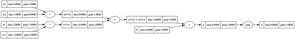
We can verify our implementation using PyTorch library

import torch
x1 = torch.Tensor([2.0]).double() ; x1.requires_grad = True # requires_grad forces the tensor to be used in calculations of gradients
x2 = torch.Tensor([0.0]).double() ; x2.requires_grad = True
w1 = torch.Tensor([-3.0]).double() ; w1.requires_grad = True
w2 = torch.Tensor([1.0]).double() ; w2.requires_grad = True
b = torch.Tensor([6]).double() ; b.requires_grad = True
n = x1*w1 + x2*w2 + b
o = torch.tanh(n)

print(o.data.item())
o.backward()

print('---')
print('x2', x2.grad.item())
print('w2', w2.grad.item())
print('x1', x1.grad.item())
print('w1', w1.grad.item())

0.0
---
x2 1.0
w2 0.0
x1 -3.0
w1 2.0

Coding a Neural Network

In the sections above, we have created a Value class that allows us to create multi-variate equations, and using back-propagation allows us to calculate gradients. For creating a neural network, we’d create the following classes that would make use of the Value class:

• Neuron – Depicting a single neuron in the network
• Layer– Depicting a single layer in the neural network that would contain multiple Neurons
• MLP– Depicting a Multi-Layer Perceptron or a neural network with multiple Layers of Neurons

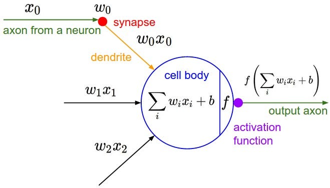
The diagram above shows the structure of a Neuron with weights(Wi), bias(b) and input(xi) as the inputs and a single output passed through an activation function tanh in our case

The weighted sum is calculated as follows: weighted_sum = (w1 * x1) + (w2 * x2) + ... + (wn * xn) Where:

• w1, w2, ..., wn: These are the weights associated with each input.
• x1, x2, ..., xn: These are the input values.

Implementing Neuron

import random
class Neuron:
 def __init__(self, ninp):
 self.w = [Value(random.uniform(-1, 1)) for _ in range(ninp)]
 self.b = Value(random.uniform(-1, 1))
 
 def __call__(self, x):
 out = sum([ wi*xi for wi, xi in zip(self.w, x)]) + self.b
 res = out.tanh()
 return res
 
 def parameters(self): # This function would be used later on while training the network
 return self.w + [self.b]

x = [1.0, 2.0, 3.0 ]
n = Neuron(3)
n(x)

---------------------------------------------------------------------------

AttributeError Traceback (most recent call last)

Cell In[123], line 3
 1 x = [1.0, 2.0, 3.0 ]
 2 n = Neuron(3)
----> 3 n(x)


Cell In[122], line 8, in Neuron.__call__(self, x)
 7 def __call__(self, x):
----> 8 out = sum([ wi*xi for wi, xi in zip(self.w, x)]) + self.b
 9 res = out.tanh()
 10 return res


Cell In[122], line 8, in <listcomp>(.0)
 7 def __call__(self, x):
----> 8 out = sum([ wi*xi for wi, xi in zip(self.w, x)]) + self.b
 9 res = out.tanh()
 10 return res


Cell In[105], line 29, in Value.__mul__(self, other)
 28 def __mul__(self, other):
---> 29 out = Value(self.data * other.data, (self, other), '*')
 31 def _backward():
 32 self.grad += other.data * out.grad


AttributeError: 'float' object has no attribute 'data'

The error above is the result of multiplying the Value type with a float type. To support such operations, we’ll modify Value with a few more methods

class Value:
 
 def __init__(self, data, _children=(), _op='', label=''):
 self.data = data
 self.grad = 0.0
 self._backward = lambda: None
 self._prev = set(_children)
 self._op = _op
 self.label = label

 def __repr__(self):
 return f"Value(data={self.data})"
 
 def __add__(self, other):
 other = other if isinstance(other, Value) else Value(other)
 out = Value(self.data + other.data, (self, other), '+')
 
 def _backward():
 self.grad += 1.0 * out.grad
 other.grad += 1.0 * out.grad
 out._backward = _backward
 
 return out

 def __mul__(self, other):
 other = other if isinstance(other, Value) else Value(other)
 out = Value(self.data * other.data, (self, other), '*')
 
 def _backward():
 self.grad += other.data * out.grad
 other.grad += self.data * out.grad
 out._backward = _backward
 
 return out
 
 def __pow__(self, other):
 assert isinstance(other, (int, float)), "only supporting int/float powers for now"
 out = Value(self.data**other, (self,), f'**{other}')

 def _backward():
 self.grad += other * (self.data ** (other - 1)) * out.grad
 out._backward = _backward

 return out
 
 def __rmul__(self, other): # other * self
 return self * other

 def __truediv__(self, other): # self / other
 return self * other**-1

 def __neg__(self): # -self
 return self * -1

 def __sub__(self, other): # self - other
 return self + (-other)

 def __radd__(self, other): # other + self
 return self + other

 def tanh(self):
 x = self.data
 t = (math.exp(2*x) - 1)/(math.exp(2*x) + 1)
 out = Value(t, (self, ), 'tanh')
 
 def _backward():
 self.grad += (1 - t**2) * out.grad
 out._backward = _backward
 
 return out
 
 def exp(self):
 x = self.data
 out = Value(math.exp(x), (self, ), 'exp')
 
 def _backward():
 self.grad += out.data * out.grad
 out._backward = _backward
 
 return out
 
 def backward(self):
 
 topo = []
 visited = set()
 def build_topo(v):
 if v not in visited:
 visited.add(v)
 for child in v._prev:
 build_topo(child)
 topo.append(v)
 build_topo(self)
 
 self.grad = 1.0
 for node in reversed(topo):
 node._backward()

'''
Trying out the above operation again
'''
x = [1.0, 2.0, 3.0 ]
n = Neuron(3)
n(x)

Value(data=-0.5181071586116809)

Next, we'll define a layer in the neural network

class Layer:
 def __init__(self, ninp, nneurons): # ninp is the number of inputs for each neuron in the layer
 self.neurons = [Neuron(ninp) for _ in range(nneurons)]
 
 def __call__(self, x):
 outs = [n(x) for n in self.neurons]
 return outs[0] if len(outs) == 1 else outs

 def parameters(self):
 return [p for neuron in self.neurons for p in neuron.parameters()]

'''
Input x is passed through each neuron of layer l, hence 4 values output from the layer
'''
x = [1.0, 2.0, 3.0 ]
l = Layer(3, 4)
l(x)

[Value(data=0.971182517031463),
 Value(data=-0.9790568300306317),
 Value(data=-0.4857385699176223),
 Value(data=-0.9636928832453497)]

Next, we'll define an MLP class that's our neural network

class MLP:
 def __init__(self, nin, nouts): # nin is the number of inputs for the first layer and nouts is an [] for output in each layer
 sz = [nin] + nouts
 self.layers = [Layer(sz[i], sz[i+1]) for i in range(len(nouts))] 

 def __call__(self, x):
 for layer in self.layers:
 x = layer(x)
 return x
 
 def parameters(self):
 return [p for layer in self.layers for p in layer.parameters()]

In the example we create the following MPL

• First layer: 3 inputs
• Middle layers: 4 and 4 outputs
• Output layer: 1

x = [2.0, 3.0, -1.0]
n = MLP(3, [4, 4, 1])
n(x)

Value(data=-0.3286322706370602)

Creating a binary classifier

For the xs as inputs, we have a target ys, which are the true predictions. We’ll create an MLP with the same structure as we saw above

xs = [
 [2.0, 3.0, -1.0],
 [3.0, -1.0, 0.5],
 [0.5, 1.0, 1.0],
 [1.0, 1.0, -1.0],
]
ys = [1.0, -1.0, -1.0, 1.0] # desired targets
n = MLP(3, [4, 4, 1])

'''
Each x in xs would be passed to MLP, resulting in ypred, this is termed as forward pass
'''
ypred = [n(x) for x in xs]
ypred

[Value(data=-0.9605353699041816),
 Value(data=-0.9652866142967272),
 Value(data=0.26960003457444665),
 Value(data=-0.9511958636250315)]

Loss

We see above that ypredi is different than yi. The difference between the values is termed as loss. We can use different methods to calculate loss. In this example, we'll make use of Squared error

loss = sum((yout - ygt)**2 for ygt, yout in zip(ys, ypred))
loss

Value(data=9.26395350181118)

draw_dot(loss)

Once we've calculated the gradient corresponding to each parameter of the MLP, we'll modify the value of each parameter by a small value also known as the learning rate

for p in n.parameters():
 p.data += -0.1 * p.grad

After updating the values, we can check the loss again; this time loss should be reduced

ypred = [n(x) for x in xs]
loss = sum((yout - ygt)**2 for ygt, yout in zip(ys, ypred))
loss

Value(data=7.829761457067251)

Training loop

We can have the above steps into a training loop

• Forward pass
• Backward pass
• Update

'''
Resetting the values
'''
xs = [
 [2.0, 3.0, -1.0],
 [3.0, -1.0, 0.5],
 [0.5, 1.0, 1.0],
 [1.0, 1.0, -1.0],
]
ys = [1.0, -1.0, -1.0, 1.0] # desired targets
n = MLP(3, [4, 4, 1])

for k in range(50):
 
 # forward pass
 ypred = [n(x) for x in xs]
 loss = sum((yout - ygt)**2 for ygt, yout in zip(ys, ypred))
 
 # backward pass
 for p in n.parameters():
 p.grad = 0.0
 loss.backward()
 
 # update
 for p in n.parameters():
 p.data += -0.1 * p.grad
 
 print(k, loss.data)

0 3.6406853121192033
1 3.610944134843126
2 3.741912394115651
3 3.2018009544051136
4 3.2524598245980503
5 1.9728216636593452
6 1.3173214047883315
7 1.0735765629752656
8 0.8890437353493715
9 0.11522009736067115
10 0.05081752438719958
11 0.03672318278028023
12 0.02979416308450841
13 0.02556184631434586
14 0.022653024581680118
15 0.02049638823502594
16 0.01881087828912575
17 0.017442066784978914
18 0.01629801693027828
19 0.015320499407445488
20 0.014470748984735923
21 0.013721869837929553
22 0.013054538143998672
23 0.012454448840696034
24 0.01191073501042354
25 0.011414954174232338
26 0.010960417756148979
27 0.010541735226885831
28 0.010154496500154066
29 0.009795045700014122
30 0.009460316742793573
31 0.009147711635699132
32 0.008855008873882249
33 0.008580293427428378
34 0.008321902472546286
35 0.00807838278062741
36 0.007848456862487212
37 0.007630995774834821
38 0.007424997058651014
39 0.007229566675831996
40 0.007043904093967112
41 0.006867289874369098
42 0.006699075268871989
43 0.00653867344237842
44 0.0063855520216464234
45 0.00623922673400612
46 0.006099255947992355
47 0.005965235965120223
48 0.005836796940995997
49 0.0057135993366707865

Inference

xs = [
 [4.0, 5.0, -3.0],
]
ypred = [n(x) for x in xs]
ypred

[Value(data=0.9658818961790056)]

Conclusion

There you have it, a working neural network that is able to learn the input data and optimize its weights using gradient descent. This article was an oversimplification of the actual neural networks, but nonetheless, it covers the operations going underneath, minus the optimizations.

I hope that through this article, you were able to improve your understanding of neural networks and dive deeper into the workings of components that you might already be familiar with.

Join thousands of data leaders on the AI newsletter. Join over 80,000 subscribers and keep up to date with the latest developments in AI. From research to projects and ideas. If you are building an AI startup, an AI-related product, or a service, we invite you to consider becoming a sponsor.

Published via Towards AI