Multivariate Linear Regression From Scratch

Author(s): Erkan Hatipoğlu

Originally published on Towards AI.

With Code in Python

Introduction

In this new episode of the Machine Learning Basics series, we will create a model for a multivariate linear regression task and validate our model using Mathplotlib, Pandas, and NumPy libraries in Python. While creating our model, we will use a Kaggle dataset as a training and validation resource. For this purpose, we will use and explain the essential parts of the following Kaggle Notebook:

Multivariate Linear Regression From Scratch

Explore and run machine learning code with Kaggle Notebooks U+007C Using data from Graduate Admission 2

www.kaggle.com

Our previous episode explained basic machine learning concepts and the notions of hypothesis, cost, and gradient descent. In addition, using Python and some other libraries, we have written functions for those algorithms and created and validated a model for a univariate linear regression task. If you are new to Machine Learning or want to refresh the basic Machine Learning concepts, reading our previous episode will be a good idea since we will not explain those subjects in this episode.

Univariate Linear Regression From Scratch

With Code in Python

pub.towardsai.net

We will use the gradient descent approach for the model creation task and will not discuss the Normal Equation since it will be the subject of another episode in this series. Therefore, we will write code for the hypothesis, cost, and gradient descent functions before training our model.

We will also introduce two new concepts: Vectorization and Feature Scaling. So, let’s start with vectorization.

Vectorization

Vectorization is the speed perspective in the implementation [1]. One way to implement Machine Learning algorithms is by using software loops in our code. Since we need to add or substruct values for each data sample for implementing Machine Learning algorithms, it seems obvious to use software loops. On the other hand, various numerical linear algebra libraries we can utilize are either built-in or quickly accessible in most programming languages. Those libraries are more efficient and can use parallel hardware in our computers if available. Therefore, instead of less efficient loops, we can use vectors and matrices in those libraries to speed up. Moreover, we will write less code resulting in a cleaner implementation [2]. This concept is known as vectorization.

This blog post will use Python’s NumPy library for vectorization.

Feature Scaling

We can speed up gradient descent by having each input value in roughly the same range [2]. This approach is called feature scaling. Applying feature scaling may be necessary for objective functions to work precisely in some machine learning algorithms or penalize the coefficients appropriately in regularization [3].

Still, for our specific case, the gradient descent may converge more quickly if we apply feature scaling since θ will descend more rapidly in small ranges than large ranges, which causes oscillations while finding the optimum θ values [2].

There are various techniques for scaling; we will present three of them:

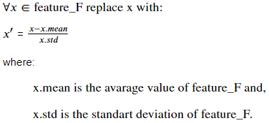
Standardization

For each sample value x of a feature, if we subtract the average value of that feature from x and divide the result by the standard deviation for that feature, we get a standardized solution. In mathematical terms:

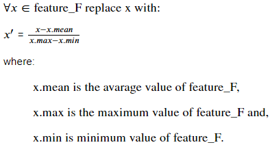
Mean Normalization

For each sample value x of a feature, if we subtract the average value of that feature from x and divide the result by the difference between the maximum and minimum values of that feature, we get a
mean normalized solution. In mathematical terms:

Min-Max Scaling

For each sample value x of a feature, if we subtract the minimum value of that feature from x and divide the result by the difference between the maximum and minimum values of that feature, we get a
min-max scaled solution. In mathematical terms:

The Normalize Function

Below you will find the code we have used for feature scaling. You can find all three approaches we have discussed in the comments. We have chosen min-max scaling for feature scaling, which you can see at the bottom of the code block.

We use the Pandas Library’s min() and max() methods inside the code block. You can refer to the Imports section for importing Pandas Library. Interested readers may also refer to the Notebook Multivariate Linear Regression From Scratch to see which columns are selected for scaling.

Imports

As stated previously, we need additional libraries to fulfill our requirements while writing the code for a multivariate regression task. These imports can be found below.

We will use the NumPy library for Matrix operations and vectorization purposes and the Pandas library for data processing tasks. The Matplotlib library will be used for visualization purposes.

Scikit-learn (or sklearn) is a prevalent library for Machine Learning. train_test_split from sklearn is used for splitting the dataset into two portions for training and validation. Although we will not use train_test_split in our code in this blog post, we need to use it for splitting our data. Interested readers may refer to the Notebook Multivariate Linear Regression From Scratch for how it is used.

The Hypothesis

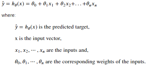
The hypothesis will compute the predicted values for a given set of inputs and weights.

The hypothesis for a linear regression task with multiple variables is of the form:

The equation above is not suitable for a vectorized solution. So let’s define θ and x column vectors such that;

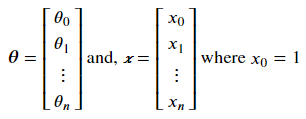
Now we can rewrite the equation above as follows:

For most of the datasets available, each row represents one training (or test) sample such that:

However, as described above, we need x₀ = 1 for a vectorized solution. So, we must adjust our data set with a new column of x₀ with all ones.

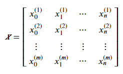
Therefore, for a dataset of m samples and n features, we can insert a new column x₀ of ones and then compute a column vector of (m x 1) dimensions such that every element of the column vector is a predicted target for one dataset sample. The formula is as follows:

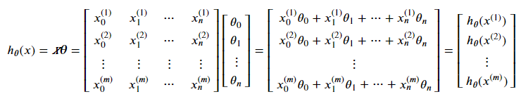
Note that we have assigned a new column x₀ to the x matrix, which is one. This is necessary for a vectorized solution, and we will see how to do it in the Model Training section.

As can be seen, we need two parameters to write the hypothesis function. These are an x matrix of (m X n+1) dimensions for training (or test) data and a θ column vector of (n+1) elements for weights. m is the number of samples, and n is the number of features. So, let’s write the Python function for the hypothesis:

Inside the hypothesis function, we return the dot product of the parameters using the NumPy library dot() method.

The Cost Function

We will use the squared error cost function as in the univariate linear regression case. Therefore, the cost function is:

To achieve a vectorized solution, we can use the following vector:

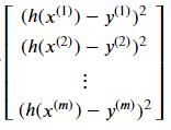
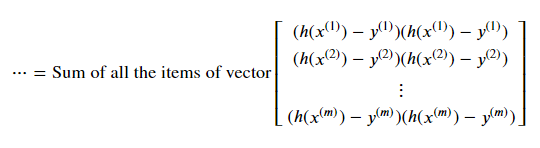
This (m X 1) vector has some resemblance to the Hypothesis vector explained above, and we will exploit this similarity. The sum of this vector’s elements is the Σ part of the cost function, and that is:

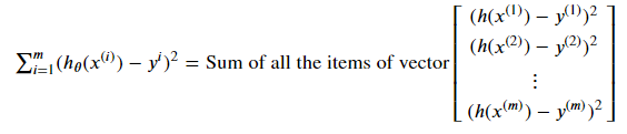
We get the vector below if we factor the squares in each vector item.

This equation can be rewritten as the dot product of the following row and column vectors.

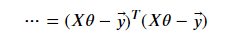
We get the following vectors if we change the ordering of the variables in the equation.

And by replacing the vectorized hypothesis with Xθ, we get the following equation.

Finally, we get the vectorized cost function by multiplying this equation with one over two times m.

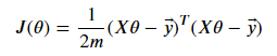
We need three parameters for the cost function: the X, y, and θ vector. The X parameter is an (m X n+1) dimensions matrix where m is the number of examples and n is the number of features, and it is the training (or test) dataset. The y parameter is an (m X 1) dimensions vector that holds the actual outputs for each sample. The θ parameter is an (n+1 X 1) dimensions vector for weights.

Note that we are using the hypothesis function inside the cost function, so to use the cost function, we must also write the hypothesis function.

We can factor the cost function formula into three parts. A constant part, a vector of (mX1) dimensions, and the transpose of the same vector with (1Xm) dimensions.

So, inside the cost function, we first calculate the constant part. Then we calculate the (mX1) vector using the hypothesis function and the y vector. We can then use NumPy’s transpose function to figure the transpose of the same vector. Finally, we can dot product the two vectors employing the Numpy library, multiply by the constant and return the result.

Gradient Descent

The gradient descent computation is identical to the univariate version, but the equation must be expanded for n + 1 weights [2].

In the formula above, n is the number of features, θⱼ (for j=0, 1, …, n) is the corresponding weights of the hypothesis function, α is the learning rate, m is the number of examples, h(x⁽ⁱ⁾) is the result of the hypothesis function for the iᵗʰ training example, y⁽ⁱ⁾ is the actual value for the iᵗʰ training example and xₖ⁽ⁱ⁾ (for k=0, 1, …, n; i=1, 2, …, m) is the value of kᵗʰ feature for the iᵗʰ training example.

Similar to what we have done in the cost function, we can rewrite the Σ part of these equations as the dot product of two vectors for j=0, 1, …, n:

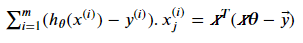
So the vectorized solution for gradient descent becomes:

As can be seen, we need four parameters for the gradient descent function: the X, y, θ vector and the learning rate α.

Note that we are using the hypothesis function inside the gradient function, so to utilize the gradient function, we must also write the hypothesis function.

Inside the function, we first compute the constant part of the equation and the transpose of X. Then, we figure out the error vector by subtracting the actual output vector from the hypothesis vector. Next, we compute the dot product of two previously calculated vectors and multiply it by the constant. As a final step, we subtract the outcome from the previous θ and return the result.

Data

To create and validate our model, we will use the following dataset [4] from Kaggle:

Graduate Admission 2

Predicting admission from important parameters

www.kaggle.com

The dataset includes several parameters critical for the application of Master’s Programs [5]:

GRE Scores ( out of 340 )
TOEFL Scores ( out of 120 )
University Rating ( out of 5 )
Statement of Purpose and Letter of Recommendation Strength ( out of 5 )
Undergraduate GPA ( out of 10 )
Research Experience ( either 0 or 1 )
Chance of Admit ( ranging from 0 to 1 )

The target variable is the ‘Chance of Admit’ parameter. We will use 80 % of the data for training and 20 % for testing. In addition, we will use a percentage estimation instead of finding the probability for the target variable. We will not explain how to load and process data. Interested readers may refer to the Notebook Multivariate Linear Regression From Scratch for loading and splitting the data.

There are two versions of CSV files in the dataset [5]. We will use version 1.1, which has 500 examples.

Model Training

Since we have written all the necessary functions, it is time to train the model.

To apply a vectorized solution, we must define an X₀ feature equal to 1 for all training examples. So our first task is to insert the X₀ column into the training and validation data. Next, we need to initialize the θ vector, and we will set weights to all zero. As the last step before gradient descent, we will assign the learning rate and threshold values.

Inside the code block, the first thing to do is compute the m and n values for training and test data. Next, we will create a list of ones to insert into the DataFrames as the first column. This is because we need to define the column X₀=1 for a vectorized solution. Next, we set the θ vector as all zeros. After initializing the learning rate and threshold values, we can calculate the initial cost value and initialize some essential variables for display purposes.

The threshold value will be used to check whether the gradient descent converges. We will subtract consecutive cost values inside the while loop to do that. If the difference is smaller than a certain threshold, we will conclude that the gradient descent converges. Otherwise, we will keep taking the gradient and recalculating the cost value.

The Result

The result below is for the initial conditions in the model training code block. The training took 24 iterations. The final cost value was computed at approximately 66, and the θ vector is calculated as:

θ: [2.03692557 1.13926025 1.14289218 6.02902784 6.60181418 6.82324225 1.20521232 1.25048269]

We can also utilize the learning curve to ensure that gradient descent works correctly [2]. The learning curve is a plot that shows us the change in the cost value in each iteration during the training, and the cost value should decrease after every iteration [2]. Interested readers may refer to the Notebook Multivariate Linear Regression From Scratch for how to plot the learning curve.

Model Validation

As explained above, we can use learning curves to debug our model. Our learning curve seems all right, and its shape is just as desired [2]. But we still require to validate our model. To do that, we can use the validation dataset, which we have split before the training starts since, for validation, we must use data that has never been used in the training process. We will use the θ vector calculated previously for validation.

The cost value of the validation dataset seems slightly bigger (worse) than the training dataset, which is expected.

Conclusion

In this blog post, we have written the hypothesis, cost, and gradient descent functions in Python with a vectorization method for a multivariate Linear Regression task. We have also scaled a portion of our data, trained a Linear Regression model, and validated it by splitting our data. We have used the Kaggle dataset Graduate Admission 2 for this purpose.

We set the learning rate high and the convergence threshold low for demonstration purposes, resulting in a learning cost of approximately 66 and a validation cost of roughly 76. This high cost is easily seen by checking the predicted and actual Chance of Admit values. By playing with the learning rate and threshold values, we can get a training cost value smaller than 20, resulting in better predictions.

But we must be aware that the dataset has been chosen only for demonstration purposes for a multivariate linear regression task, and there may be far better algorithms for this dataset.

Interested readers can find the code used in this blog post in the Kaggle notebook Multivariate Linear Regression from Scratch.

Thank you for reading!

References

[1] Ng, A. and Ma, T. (2022) CS229 Lecture Notes, CS229: Machine Learning. Stanford University. Available at: https://cs229.stanford.edu/notes2022fall/main_notes.pdf (Accessed: December 24, 2022).

[2] Ng, A. (2012) Machine Learning Specialization, Coursera.org. Stanford University. Available at: https://www.coursera.org/specializations/machine-learning-introduction (Accessed: January 9, 2023).

[3] Feature scaling (2022) Wikipedia. Wikimedia Foundation. Available at: https://en.wikipedia.org/wiki/Feature_scaling (Accessed: March 6, 2023).

[4] Mohan S Acharya, Asfia Armaan, Aneeta S Antony: A Comparison of Regression Models for Prediction of Graduate Admissions, IEEE International Conference on Computational Intelligence in Data Science 2019

[5] Acharya, M.S. (2018) Graduate admission 2, Kaggle. Available at: https://www.kaggle.com/datasets/mohansacharya/graduate-admissions (Accessed: March 14, 2023).

Join thousands of data leaders on the AI newsletter. Join over 80,000 subscribers and keep up to date with the latest developments in AI. From research to projects and ideas. If you are building an AI startup, an AI-related product, or a service, we invite you to consider becoming a sponsor.

Published via Towards AI