


How does “Stable Diffusion” Really Work? An Intuitive Explanation
Last Updated on November 6, 2023 by Editorial Team
Author(s): Oleks Gorpynich
Originally published on Towards AI.
“Stable Diffusion” models, as they are commonly known, or Latent Diffusion Models as they are known in the scientific world, have taken the world by storm, with tools like Midjourney capturing the attention of millions. In this article, I will attempt to dispel some mysteries regarding these models and hopefully paint a conceptual picture in your mind of how they work. As always, this article won’t reach into the pit of details, but I will provide some links at the end that do. The paper, which lies as the main information source behind this article, will be the first link included.
Motivation
There are a few approaches to image synthesis (creating new images from scratch), and they include GANs, which perform poorly on diverse data; Autoregressive Transformers, which are slow to train and execute (similar to LLM transformers generating text token by token, they generate images patch by patch), and diffusion models which by themselves counter some of these issues, but yet remain computationally expensive. It still takes hundreds of CPU days to train these, and actually utilizing the model involves running it step by step to produce a final image, which also takes considerable time and compute.
Quick Overview of Diffusion Models
To understand how Diffusion models work, let’s first look at how they are trained, which is done in a slightly nonintuitive way. We begin by applying noise to an image repeatedly, which creates a “Markov chain” of images. In such a way, we are able to get some number T of repeatedly more noisy images from a singular original image.
Our model then learns to predict the exact noise that was applied at a certain time step, and we can use its output to “denoise” the image at that time step. This effectively allows us to go from image T to image T-1. To reiterate, the model is trained by giving it the image with noise applied at some time T, and the time T itself, and the output is what noise was applied to bring it from time T-1 to T!
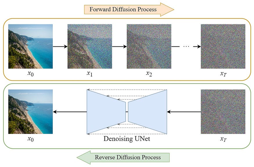
Once we have such a model trained, we can repeatedly apply it to random noise to produce a new, novel image. The great article by the wonderful
Steins where the above image is from explains this in more depth.
UNet Model
The model that is commonly used to predict the noise at each time step is a “UNet” architecture model. This is a type of architecture that repeatedly applies Convolutional layers, pooling layers, and skip connections to first downscale an image but increase depth (feature maps), and then transposed convolutions are used to up-sample the feature maps back to the original image dimensions. Here is a great article by
Maurício Cordeiro that explains this model in greater depth.
Issues
This is where the issues of traditional diffusion models come out. The first issue is training time. Assuming we have N images, and we apply noise to an image T times, that is N*T possible inputs to our model. And often times, these are high-resolution images, and each input would incorporate the large image dimensions. After all, we don’t want Midjourney to produce pixel art…
And then, assuming we do have our model trained, to get back from random noise to an image, we must apply the weights T times repeatedly! Remember, our model is only able to give us the image from the previous time step, and we must get from time step T to time step 0.
The other issue lies in the utility of such a model. If you noticed, input text wasn’t mentioned once yet; however, we are all used to implementations converting text to images, not random noise to images. So, how and where exactly does this feature come in?
Latent Diffusion Models
A key idea that would fix these issues is splitting our model into two separate ones.
The first model is trained to encode and decode images into a “latent space” which retains a lot of the “perceptual” details behind the image, but reduces the data dimensions. As a way to intuitively understand this, one can think of some noise in images that we really don’t have to learn (a blue sky with pixels slightly changing their hue).
The second model is the actual Diffuser, which can convert this latent space representation into an image. However, this Diffuser has a special modification that allows it to “understand” and be directed by inputs from other domains, such as text.
Perceptual Image Compression
Let’s begin with the first model — the image encoder/decoder. Remember, the idea is to prepare images for the actual Diffuser in such a way that important information is preserved while dimensions are decreased.
This compression model is actually called an “autoencoder”, and again this model learns to encode data into a compressed latent space and then decode it back to its original form. The goal of such a model is to minimize the difference between the input and the reconstructed output. For our loss function, we use two components.
- Perceptual Loss — Our goal is to minimize the differences in image features (such as edges or textures), as opposed to pixel differences between the original and decoded versions. There are existing tools that can extrapolate these from images, and we can use these.
- Patch-based Adversarial Objective — A GAN (check out my previous article on different types of models) whose goal is to enforce local realism, analyzing the image patch by patch and classifying whether a certain patch is real or fake.
This has the additional benefit of avoiding blurring, as what we are optimizing for isn’t pixel difference but feature difference. This means that if our model produced an image that is slightly different in pixel coloring but still retains the same “features”, it won’t be penalized much and this is what we want. However, if the pixel colorings are close to each other, but the features are off, the model will be penalized quite a bit (hence the blurring part). Effectively, this prevents the decoder (and by extension, the final Diffuser) from “cheating” and creating images with pixel values that are close to the original data set, but actual features that are “off”.
Text
So where and how does text factor into this?
When training our model, we not only train it to diffuse images (or, more accurately the latent space representations of these images produced by our first model), we also train it to understand the text and learn to use certain parts of the text to generate these images. This is because “cross attention”, the mechanism which allows the model to selectively focus on certain text features or aspects, is built into the model itself. Here is a diagram showcasing this.
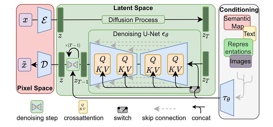
Through a separate encoder, the text is converted into an “intermediate representation” (a representation in which more important parts of the text have more weight), and these weights affect the layers of the UNet, directing the final image that will be produced. This is because the model has a “cross attention” component built in which, similarly to transformers, allows different parts of the intermediate representation to affect certain parts of the image less and others more. This is, of course, trained through a standard forward-propagation and back-propagation scheme. Our Denoising UNet is fed the text and some random noise (both encoded), and its final output is compared to the original image. The model both learns to use the text effectively and denoise effectively at the same time. If you aren’t familiar with forward and backpropagation, I highly recommend looking into these topics, as they are fundamental to machine learning.
Conclusion
LDMs perform well on all kinds of tasks, including inpainting, super — resolution, and image generation. This powerful model has become a mainstay in the AI graphics world, and we are still discovering new use cases. And although this article should give you a conceptual understanding, there are a lot more details to this. If you would like to learn more, check out this paper called “High-Resolution Image Synthesis with Latent Diffusion Models” which describes the math behind a lot of the things I mentioned.
Sources
- https://openaccess.thecvf.com/content/CVPR2022/papers/Rombach_High-Resolution_Image_Synthesis_With_Latent_Diffusion_Models_CVPR_2022_paper.pdf
- https://medium.com/@steinsfu/diffusion-model-clearly-explained-cd331bd41166
- https://medium.com/analytics-vidhya/creating-a-very-simple-u-net-model-with-pytorch-for-semantic-segmentation-of-satellite-images-223aa216e705
Join thousands of data leaders on the AI newsletter. Join over 80,000 subscribers and keep up to date with the latest developments in AI. From research to projects and ideas. If you are building an AI startup, an AI-related product, or a service, we invite you to consider becoming a sponsor.
Published via Towards AI
Towards AI Academy
We Build Enterprise-Grade AI. We'll Teach You to Master It Too.
15 engineers. 100,000+ students. Towards AI Academy teaches what actually survives production.
Start free — no commitment:
→ 6-Day Agentic AI Engineering Email Guide — one practical lesson per day
→ Agents Architecture Cheatsheet — 3 years of architecture decisions in 6 pages
Our courses:
→ AI Engineering Certification — 90+ lessons from project selection to deployed product. The most comprehensive practical LLM course out there.
→ Agent Engineering Course — Hands on with production agent architectures, memory, routing, and eval frameworks — built from real enterprise engagements.
→ AI for Work — Understand, evaluate, and apply AI for complex work tasks.
Note: Article content contains the views of the contributing authors and not Towards AI.
Related posts
Recent Posts

")


