How did Binary Cross-Entropy Loss Come into Existence?

Author(s): Towards AI Editorial Team

Originally published on Towards AI.

Exploring the Genesis of Binary Cross-Entropy Loss Function

Author(s): Pratik Shukla

“You always pass failure on the way to success.” — Mickey Rooney

Table of Contents:

1. Introduction
2. Properties of the binary classification problem
3. Basics of Bernoulli trials
4. Probability of multiple independent events
5. Properties of logarithm
6. Why do we take a log of Bernoulli trails
7. Why do we take the negative log of Bernoulli trials
8. Single Bernoulli trial
9. Multiple independent Bernoulli trials
10. Scaling a function
11. Conclusion
12. References and resources

Introduction:

In this tutorial, we will derive the equation of the binary cross-entropy loss. The equation of the binary cross-entropy loss is given as follows.

We will start with a single Bernoulli trial and make our way through the complicated mathematical formulas involved to derive the equation of the binary cross-entropy loss. Let’s start!

The Binary Cross-Entropy Loss function is a fundamental concept in the field of machine learning, particularly in the domain of deep learning. It is a mathematical function that measures the difference between predicted probabilities and actual binary labels in classification tasks. The Binary Cross-Entropy Loss function has become a staple in the training of neural networks, but its origins and development are not always well-known. In this blog, we will explore the history and evolution of the Binary Cross-Entropy Loss function, delving into its origins and discussing its applications in modern machine learning. By understanding the history of this crucial function, we can gain a better understanding of its purpose and potential for future research.

Properties of binary classification problem:

Each binary classification problem has the following properties:

1. Each example of the binary classification dataset belongs to one of the two complimentary classes.
2. The result of one example does not affect the result of any other examples. It means that each example is independent of the other.
3. All the examples are generated from the same underlying distribution.

In probability theory, if a dataset follows the 2nd and 3rd properties, then the examples are said to be independent and identically distributed (i.i.d). Considering the i.i.d. nature of the data helps to make the calculations much more straightforward.

Basics of Bernoulli trials:

Now, in binary classification problems, we have to predict the value only for one class because the probability of the negative class can be easily derived from it. It means that suppose we are performing a binary classification problem, and our outputs are dog or cat. We only need to predict the probability of a particular example being a dog. The probability of that specific example being a cat can be easily derived from it.

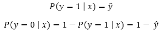
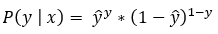
We can summarize this concept using the following formula.

Here we know that ŷ is the predicted value. A good binary classifier should produce a high value of ŷ (ideally 1) when the example has a positive label (y=1). Also, it should produce a low value of ŷ (ideally 0) when the example has a negative label (y=0). So, our goal should be the following.

Produce a high value of ŷ when y=1

Produce a low value of ŷ when y=0

Next, based on that, we can say that we need to maximize ŷ when y=1, and we need to minimize ŷ when y=0. We can say the same thing in other words as well.

Maximize ŷ when y=1

Maximize 1-ŷ when y=0

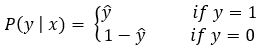
Instead of having two different equations for the positive and negative classes, we can create a simplified version that works for both classes.

The single-line expression shown in the above figure is known as a Bernoulli trial. We need to calculate it for each of the data points. After we have the results for each Bernoulli trial, we can get the final result by their multiplication.

Probability of multiple independent events:

For independent events, we can say the following.

Properties of logarithm:

1. Product rule:

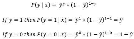
2. Power rule:

Why do we take a log of Bernoulli trials?

Alright! So, as of now, we have arrived at the following equation.

Now, as we have discussed, we will have to find the value of each Bernoulli trial. After we have the value of each Bernoulli trial, we will find their product of them. Now, we know that since ŷ is the probability value, its value will always be between 0 and 1. So, when we multiply many values between 0 and 1, the final product might get infinitesimal or next to zero. So, to avoid this problem, we usually perform the log operation. Here note that the product rule of logarithms converts the multiplication into summation. So, instead of finding the product of values between 0 and 1, we find their summation. This is how we can avoid the problem of getting 0 as an output every time.

Now, let’s take an example to understand it in a better way.

We can see this problem and its solution in the following example.

Why do we take a negative log of Bernoulli trial?

Alright! So, after applying the natural logarithm to the Bernoulli Distribution equation, we get the following equation.

Here, note that y is the actual label of the data, and y can take only one of the two possible values (0 or 1). The equation basically gives us the loss value. Remember that our ultimate goal is to find the optimum loss value (ideally 0).

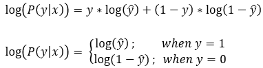
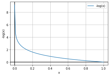
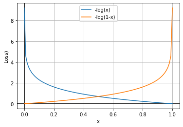
Based on the above equation, we can say that we have to minimize the value of log(ŷ) and log(1-ŷ). Now we know that ŷ represents the value of probability, so the value of ŷ can be in the interval of [0,1]. Now, let’s plot the graph of log(ŷ) and log(1-ŷ).

Here, our goal is to find the optimum loss value, which should ideally be 0. So, from the graphs, we can see that we have to maximize the function to find the optimum values here. We generally try to minimize the function or use the gradient descent algorithm in the machine learning algorithm. But, as shown in the above graphs, the curves are concave. So, here we’ll have to use the gradient ascent algorithm to reach the optimal points.

To keep the standard convention of using the gradient descent algorithm, we find the negative of the log function. So, instead of finding the function’s maximum, we will find the minimum of the function. Let’s see how it works.

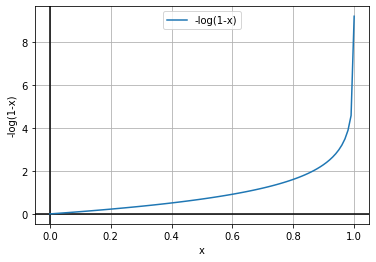
In the above graphs, we can see that we will find the optimum values at the minimum of the graphs. So, here we can use the gradient descent algorithm to find the optimal parameters.

Before we move on to multiple individual Bernoulli trials, let’s first see how this concept works for a single Bernoulli trial.

Single Bernoulli Trial:

Step — 1: Applying log

Here we are taking the original formula and applying a log to it.

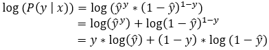
After applying the natural log to the Bernoulli Distribution, our formula is simplified into a sum of the log of probabilities.

Step — 2: Finding the negative of log

Next, we are finding the negative of the above-given formula.

Multiple Independent Bernoulli Trials:

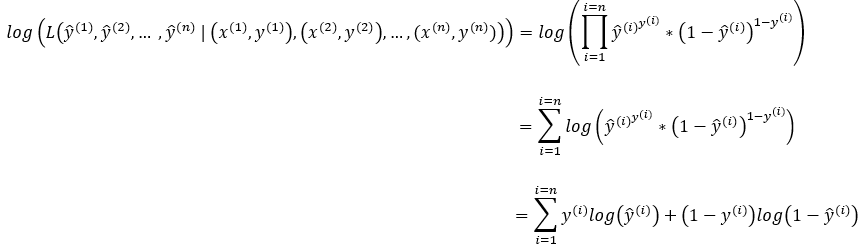
Next, we have to apply this concept to multiple independent Bernoulli trials. As we discussed before, we will need to find the product of the probabilities of each independent Bernoulli trial.

Step — 1: Applying log

Next, we will apply the log to the product of the probabilities of each independent Bernoulli trial. Here note that using the log converts the product into summation.

Step — 2: Finding the negative of log

Next, we will find the negative log of the probabilities of each independent Bernoulli trial.

Scaling a Function:

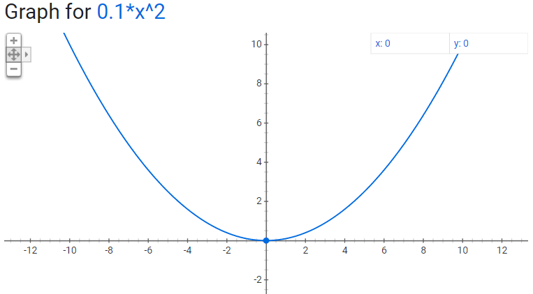
Now, let’s understand how scaling a function does not change its maximum or minimum point with the help of an example. Let’s say our function is y=X². Now, we will scale this function by a factor of k. Let’s see the graphs of the original and scaled functions to find the minimum point for each.

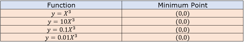
Here we can see that scaling a function does not change its maximum or minimum point. Now, let’s plot the graphs of these functions to look visually at them.

We can see that scaling a function does not change its minimum or maximum points. Now, we will divide our log-likelihood function by our dataset’s total number of examples (n).

The above formula is known as the Binary Cross Entropy function.

Conclusion:

In conclusion, the Binary Cross-Entropy Loss function has become a critical component of modern machine learning, particularly in deep learning applications. Its origins can be traced back to the early days of information theory and statistical learning, where researchers were interested in measuring the accuracy of classification models. Over the years, the Binary Cross-Entropy Loss function has undergone significant development and refinement, leading to its current widespread use in training neural networks. By understanding the history and evolution of this important function, we can gain a deeper appreciation for its purpose and potential for future research. As machine learning continues to evolve, it is likely that the Binary Cross-Entropy Loss function will continue to play a crucial role in advancing the field.

Citation:

For attribution in academic contexts, please cite this work as:

Shukla, et al., “How did Binary-Cross Entropy Loss Come into Existence?”, Towards AI, 2023

BibTex Citation:

@article{pratik_2023, 
 title={How did Binary Cross-Entropy Loss Come into Existence?}, 
 url={https://pub.towardsai.net/probability-vs-likelihood-a79335c985f7}, 
 journal={Towards AI}, 
 publisher={Towards AI Co.}, 
 author={Pratik, Shukla},
 editor={Binal, Dave}, 
 year={2023}, 
 month={Mar}
}

References and Resources:

1. Binary Entropy Function

Join thousands of data leaders on the AI newsletter. Join over 80,000 subscribers and keep up to date with the latest developments in AI. From research to projects and ideas. If you are building an AI startup, an AI-related product, or a service, we invite you to consider becoming a sponsor.

Published via Towards AI