Heteroscedasticity and Homoscedasticity in Regression Learning

Author(s): Jose D. Hernandez-Betancur

Originally published on Towards AI.

Variability of the residual in regression analysis

1. Introduction

In data science and statistical analysis, several challenges can appear during the modeling process, making it difficult to get high-performance models. One of those challenges is the instability or high variability of residuals or errors, which is known as heteroscedasticity. In this article, we will explore exactly what heteroscedasticity is and how it can negatively affect the performance of data-driven models. In addition, we will introduce techniques commonly used to identify heteroscedasticity and strategies that are part of the arsenal that statisticians and data scientists have to tackle this problem. Join me through this article on heteroscedasticity so that you can include it in your data science and statistical terms and gain insights for future projects.

2. What Heteroscedasticity and Homoscedasticity are?

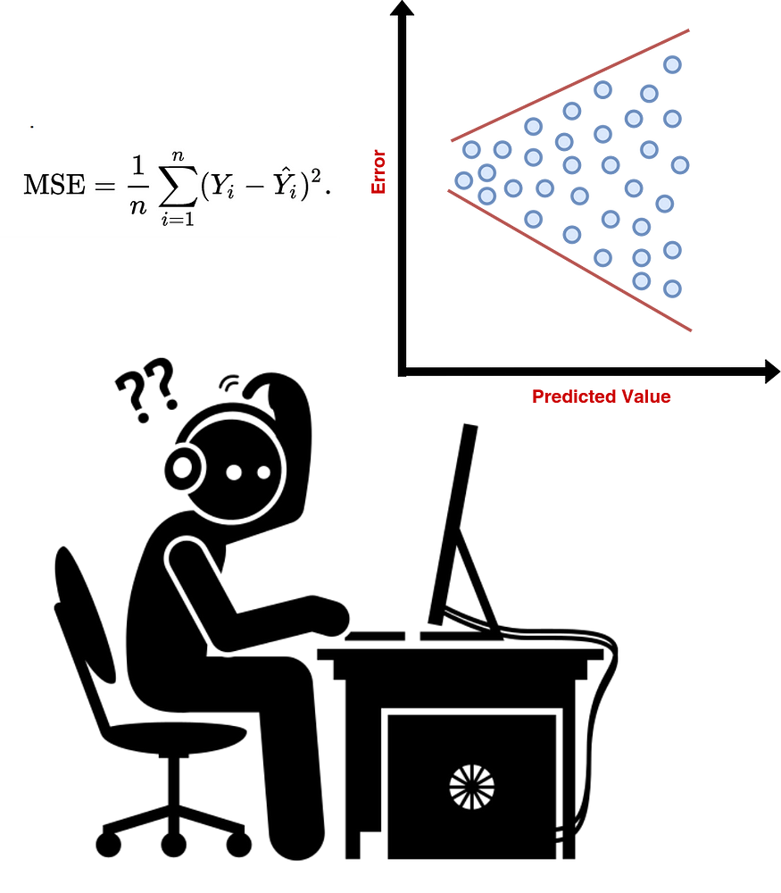
A data science practitioner or statistician uses the term heteroscedasticity to refer to situations during modeling or statistical analysis in which the variability or dispersion of the error or residual in a data-driven model is not constant across the range of predictor variables. In contrast, homoscedasticity, or constant variance, implies that the variability of the errors remains consistent across the predictor domain.

Heteroscedasticity violates one of the key assumptions of regression analysis, which assumes homoscedasticity. Thus, if heteroscedasticity occurs, the ordinary least squares estimates may be biased, inefficient, and unreliable.

The presence of heteroscedasticity can lead to biased parameter estimates, either inflated or deflated standard errors, and incorrect hypothesis testing results. It can lead to erroneous inferences and impact the overall validity and interpretability of the model.

3. How to Detect Heteroscedasticity?

Now, in this section, let’s use Python to explore two techniques widely used to detect heteroscedasticity. One simple alternative is graphical, while the other is based on inferential statistics:

• Graphical technique: The graphical tool used to detect heteroscedasticity is the residual plot. The x-axis of the plot represents the predicted values or independent variables, while the y-axis represents the residuals or errors. A well-behaved residual plot for homoscedasticity typically exhibits no outliers, a zero mean (i.e., a cluster around zero), no clear pattern or trend (i.e., a random pattern), and is relatively consistent across the range of predicted values (i.e., a constant spread).
• Inferential technique: Statisticians have developed different inferential techniques to draw conclusions about heteroscedasticity. In this article, we will use the Breusch–Pagan test to determine whether the variance of the residuals depends on the predictor variable. In this test, the null hypothesis is homoscedasticity, while the alternative (or research) hypothesis states heteroscedasticity (i.e., the variance of residuals is dependent on the predictor variables).

A Simple Test for Heteroscedasticity and Random Coefficient Variation on JSTOR

T. S. Breusch, A. R. Pagan, A Simple Test for Heteroscedasticity and Random Coefficient Variation, Econometrica, Vol…

www.jstor.org

3.1. Data Generation

Now, to start with the example in Python, let’s import the libraries required numpy, matplotlib, statsmodels, and scipy (for later). Let’s generate two datasets, each with 100 examples. One of the datasets will suffer from heteroscedasticity, while the other satisfies the homoscedasticity assumption.

# Import libraries
import numpy as np
import matplotlib.pyplot as plt
import statsmodels.api as sm
from statsmodels.stats.diagnostic import het_breuschpagan

# Set the random seed for reproducibility
np.random.seed(0)

# Number of data points
n = 100

# Define predictor variable (heteroscedasticity)
X_het = np.linspace(1, 11, n)

# Define outcome variable relationship (heteroscedasticity)
epsilon = np.random.normal(0, 1, size=100)
y_het = X_het + epsilon * (1 + X_het/5)

# Define predictor variable (homoscedasticity)
X_hom = np.linspace(-5, 5, n)

# Define outcome variable relationship (homoscedasticity)
y_hom = np.random.normal(loc=0, scale=np.ones_like(X_hom) * 2, size=n)

3.2. Base Model Fitting

The code snippet presented below is a function that trains an ordinary least squares (OLS) regression based on a dataset and returns the fitted model.

def fit_model(X, y):
 """
 Fit your regression model and obtain residuals

 Arguments:
 - X: independent variable
 - y: dependent variable

 Output:
 - model: trained model
 """

 model = sm.OLS(y, sm.add_constant(X)).fit()

 return model

Thus, with the above function, let’s train different models using the OLS algorithm. The first model is trained on the dataset with heteroscedasticity (model_het), while the second one is trained on the dataset with homoscedasticity (model_hom).

# Fit the model (heteroscedasticity)
model_het = fit_model(X_het, y_het)

# Fit the model (homoscedasticity)
model_hom = fit_model(X_hom, y_hom)

3.2. Residual Plot

Now, we can create a function that receives the trained model as input so that it can plot the residuals or errors (y-axis) against the fitted or predicted values (x-axis). The code snippet below presents the resulting Python function to generate the residual plot.

def plot_residual(model):
 """
 Plot residuals against predicted values

 Arguments:
 - model: trained model

 Output:
 None
 """

 residuals = model.resid

 fig, ax = plt.subplots()
 ax.scatter(model.fittedvalues, residuals, alpha=0.8)
 ax.axhline(y=0, color='red', linestyle='--', label='Horizontal Line')
 ax.set_xlabel("Predicted values", fontweight='bold')
 ax.set_ylabel("Residuals", fontweight='bold')
 ax.set_title("Residual plot for heteroscedasticity", fontweight='bold')
 ax.grid(color='lightgray', linestyle='--')
 plt.show()

Using the function for the residual plot generation and running the following code line, let’s generate the residual plot for the dataset with heteroscedasticity:

# Check residual plot (heteroscedasticity)
plot_residual(model_het)

Similarly, let’s do the same for the dataset with homoscedasticity by running the below code snippet:

# Check residual plot (homoscedasticity)
plot_residual(model_hom)

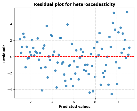
As can be seen in Figure 2, the residuals for the dataset with predicted homoscedasticity are normally distributed around the zero line. The consistency of the error over the range of projected values can also be established. Under the homoscedasticity assumption, the ideal behavior of the residual plot is characterized by a random distribution with no outliers, a constant spread, and no apparent trend. Figure 1, however, shows that the error is essentially non-zero for predicted values below 3. The same holds true for numbers above 10. This demonstrates heteroscedasticity (which is to be expected given our case), as seen above.

3.3. Breusch-Pagan Test

The residual plot is a useful method, but it requires a manual approach in which the practitioner must carefully examine the patterns displayed on the plot. For this reason, it is helpful to have a method that, when incorporated into an automated experiment, allows a Python program to automatically infer results based on testing rules. As mentioned earlier, the Breusch–Pagan test will aim at statistical inferential-based analysis. The below figure shows the Python implementation for the hypothesis test. alpha is the level of significance, which by default is 0.05.

def breusch_pagan_test(model, X, alpha=0.05):
 """
 Perform Breusch-Pagan test

 Arguments:
 - X: independent variable
 - model: trained model

 Output:
 None
 """

 residuals = model.resid
 p_value = het_breuschpagan(residuals, sm.add_constant(X))[1]

 print("Breusch-Pagan test p-value: ", p_value)
 print("Any evidence of heteroscedasticity?: ", p_value < alpha)

Let’s apply the aforementioned function to the heteroscedastic dataset. To see the results of the tests on your screen, run the following line:

# Check Breusch-Pagan test (heteroscedasticity)
breusch_pagan_test(model_het, X_het)

Breusch-Pagan test p-value: 0.007785481845777098

Any evidence of heteroscedasticity?: True

Similarly, let’s execute this code to get the outcomes for the homoscedastic dataset:

# Check Breusch-Pagan test (homoscedasticity)
breusch_pagan_test(model_hom, X_hom)

Breusch-Pagan test p-value: 0.8104035079011154

Any evidence of heteroscedasticity?: False

The p-value for the dataset is, as expected, lower than the level of significance, being less than 0.05 for the heteroscedastic dataset. That is, there is statistical proof that this dataset is subject to heteroscedasticity. In contrast, the alternative hypothesis is rejected for the homoscedastic dataset since there is no statistical evidence to support the idea that the data is heteroscedastic rather than homoscedastic.

4. How to Handle Heteroscedasticity?

The aforementioned methods and findings are both theoretically and practically intriguing. Even if you’ve established heteroscedasticity using one of the above approaches or another, you may still be wondering what to do next. Well, depending on the peculiarities of your case and analysis, a variety of several methods may be useful additions to your toolkit. The following are some common methods for handling heteroscedasticity in regression, as well as some resources worth consulting for further details:

• Transformation:

• Weighted Least Squares (WLS) Regression:

When and How to use Weighted Least Squares (WLS) Models

WLS, OLS’ Neglected Cousin

towardsdatascience.com

By

Jonathan Balaban

• Robust Standard Errors:

University of Virginia Library Research Data Services + Sciences

Collections, services, branches, and contact information.

data.library.virginia.edu

• Generalized Least Squares (GLS) Regression:

Generalized Least Squares (GLS): Mathematical Derivations & Intuition

Introduction to GLS with relations to OLS & WLS

towardsdatascience.com

By

Andrew Rothman

• Data Stratification or Segmentation:

When important variables for describing the problem are missing or misspecified, good variable selection and data collection may help reduce heteroscedasticity in addition to the aforementioned strategies.

4.1. Yeo-Johnson transformation

Using transformations like the logarithmic one helps normalize skewed data in ML by minimizing the impact of extreme results. In order to generate a more linear relationship between variables, transformations are sometimes used. For curved or nonlinear relationships, transformation can aid with visualization and interpretation. In addition to the aforementioned benefits, transformations are frequently employed to deal with heteroscedasticity by reducing the variance of the dependent variable. Therefore, the Yeo-Johnson transformation, an alternative method for reducing heteroscedasticity, will be implemented in this article. This transformation allows for the processing of data with a wide variety of distributions, the transformation of both positive and negative values, and the mitigation of the effect of outliers (see link below for more infoU+1F447).

The Box-Cox and Yeo-Johnson transformations for continuous variables

The Box-Cox and Yeo-Johnson transformations are two different ways to transform a continuous (numeric) variable so that…

statisticaloddsandends.wordpress.com

Let’s put this solution into action in Python and evaluate the transformed results. Yeo-Johnson transformation is included in the scipy package, and after applying it, the OLS can be fitted:

# Import libraries
import scipy.stats as stats

# Apply the Yeo-Johnson transformation to the dependent variable
y_het_yeojohnson, lambda_ = stats.yeojohnson(y_het)

# Fit the model (after transformation)
model_het_yeojohnson = fit_model(X_het, y_het_yeojohnson)

Now, let’s check the results, considering the graphical and statistical tests introduced previously:

# Check residual plot (after transformation)
plot_residual(model_het_yeojohnson)

# Check Breusch-Pagan test (after transformation)
breusch_pagan_test(model_het_yeojohnson, X_het)

After applying the transformation to the heteroscedastic dataset, the error values are much closer to zero, as illustrated in Figure 3. The apparent shift of the error distribution to a zero or x-axis-normal distribution. But the graphical representation is not entirely obvious. The p-value for the Breusch-Pagan test is greater than 0.05; hence, the null hypothesis isn’t rejected. Thus, following the Yeo-Johnson transformation, heteroscedasticity has been reduced.

Breusch-Pagan test p-value: 0.5518034761699758

Any evidence of heteroscedasticity?: False

Conclusion

We use the idea of heteroscedasticity and its consequences, especially in homoscedasticity-assumptive models, to our advantage in this work. We use a graphical tool called a residual plot to investigate heteroscedasticity, and we introduce a statistical inference tool called a Breusch-Pagan test, both of which help us assess whether or not there is sufficient evidence to conclude that heteroscedasticity does, in fact, occur. Furthermore, we present methods for handling heteroscedasticity, and in particular, we employed the Yeo-Johnson transformation, which is adaptable to a wide range of data distributions and values. Breusch-Pagan test results showed that heteroscedasticity could be reduced by utilizing the transformation method.

Despite its popularity in discussions of linear regression, heteroscedasticity can also be seen in the residuals or prediction errors of other machine-learning techniques. Such methods include regression based on the Gaussian process, time series analysis, artificial neural networks, support vector machines, and tree-based algorithms.

If you enjoy my posts, follow me on Medium to stay tuned for more thought-provoking content, clap this publication U+1F44F, and share this material with your colleagues U+1F680…

Get an email whenever Jose D. Hernandez-Betancur publishes.

Get an email whenever Jose D. Hernandez-Betancur publishes. Connect with Jose if you enjoy the content he creates! U+1F680…

medium.com

Suggested Material

• W. Rutha and T. Loughin, The Effect of Heteroscedasticity on Regression Trees (2016), arXiv (Cornell University)
• Q. Le, A. Smola and S. Canu, Heteroscedastic Gaussian Process Regression (2020)
• H. Park and C. Hwang, Weighted Support Vector Machines for Heteroscedastic Regression (2006), Journal of the Korean Data and Information Science Society
• A. Stirn, Faithful Heteroscedastic Regression with Neural Networks (2022), arXiv (Cornell University)
• V. Cerqueira, How to Detect Heteroskedasticity in Time Series (2022), Towards Data Science

Join thousands of data leaders on the AI newsletter. Join over 80,000 subscribers and keep up to date with the latest developments in AI. From research to projects and ideas. If you are building an AI startup, an AI-related product, or a service, we invite you to consider becoming a sponsor.

Published via Towards AI