Deep Learning from Scratch in Modern C++: Gradient Descent

Author(s): Luiz doleron

Originally published on Towards AI.

Let’s have fun by implementing Gradient Descent in pure C++ and Eigen.

In this story, we will cover the fitting of 2D convolution kernels from data by introducing the Gradient Descent algorithm. We will use convolutions and the concept of cost functions introduced in the previous story coding everything in modern C++ and Eigen.

About this series

In this series, we will learn how to code the must-to-know deep learning algorithms such as convolutions, backpropagation, activation functions, optimizers, deep neural networks, and so on, using only plain and modern C++.

This story is: Gradient Descent in C++

Check other stories:

0 — Fundamentals of deep learning programming in Modern C++

1 — Coding 2D convolutions in C++

2 — Cost Functions using Lambdas

4 — Activation Functions

… more to come.

Function Approximation as an Optimization Problem

If you read our previous talk, you already know that, in machine learning, we are most of the time concerned with using data to find function approximations.

Usually, we obtain function approximations by finding the coefficients which minimize the cost value. Thus, our approximation problem is converted into an optimization problem where we try to minimize the value of a cost function.

Cost Functions and Gradient Descent

Cost functions compute the cost of using a function H(X) to approximate the target function F(X). For example, if H(X) is the convolution between the input X and the kernel k, the MSE cost function is given by:

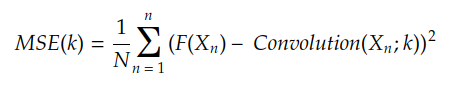
We usually do Yₙ = F(Xₙ) which results in:

MSE is the Mean Squared Error, the cost function introduced in the previous story

Thus, our objective is to find the kernel values kₘ which minimizes MSE(k). The most basic (but powerful) algorithm to find kₘ is Gradient Descent.

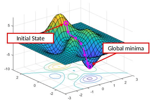
Gradient Descent uses the cost function gradients to find the minimum cost. In order to understand what gradients are, let’s talk about the cost surface.

Plotting the cost surface

To make it easier to understand, let’s assume for a moment that the kernel k consists of only two coefficients [k00, k01]. If we plot the value of MSE(k) for each possible combination of [k00, k01] we will end up with a surface like this:

At each point (k00, k01, MSE(k00, k01)) , the surface has an inclination angle with the 0k₀₀ axis and another inclination angle with the 0k₀₁ axis:

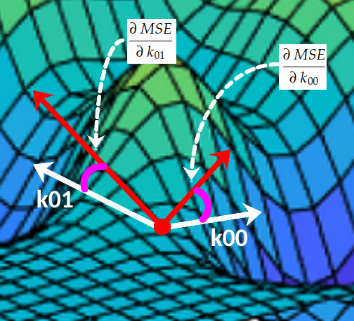
These two slopes are the partial derivatives of the MSE curve with respect to axes Ok₀₀ and Ok₀₁, respectively. In Calculus, we very use the symbol ∂ to denote partial derivatives:

Together, these two partial derivatives form the gradient of MSE with respect to axes Ok₀₀ and Ok₀₁. This gradient is used to drive the execution of our gradient descent algorithm illustrated below:

The algorithm which performs this “navigation” over the cost surface is called Gradient Descent.

Gradient Descent

The gradient descent pseudocode is described below:

gradient_descent:

 initialize k, learning_rate, epoch = 1

 repeat
 k = k - learning_rate x ∇Cost(k)
 until epoch <= max_epoch

 return k

The value of learning_rate x ∇Cost(k) is usually called weight update. We can resume the behavior of gradient descent by:

for each iteration:
 calculate the weight update
 subtract it from the parameter k

As its name indicates, Cost(k) is the cost function for a configuration k. The objective of gradient descent is to find the value of k in which Cost(k) is minimum.

learning_rate is usually a scalar like 0.1, 0.01, 0.001 or so. This value controls the step size during the optimization process.

The algorithm loops for max_epoch times. Occasionally, we stop the algorithm earlier, i.e., even if epoch < max_epoch, in cases where Cost(k) is too small.

We usually refer to parameters like learning_rate and max_epoch by the name of hyperparameters.

The last thing that we need to know to implement gradient descent is how to calculate the gradient of C(k). Fortunately, in the case of the cost function being MSE, finding ∇Cost(k) is pretty straightforward, as discussed ahead.

Finding the MSE gradients

We have seen so far that the gradient’s components are the slope of the cost surface for each axis 0kᵢⱼ. We also have seen that the gradient of MSE(k) with respect to each i-th, j-the coefficient of the kernel k is given by:

Let’s remember that MSE(k) is given by:

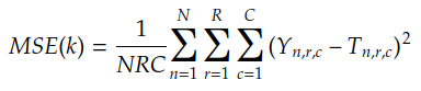
where n is the index of each pair (Yₙ, Tₙ), and r & c are the indexes of the output matrix coefficients:

Using the chain rule and the linear combination rule we can find the MSE gradient in the following way:

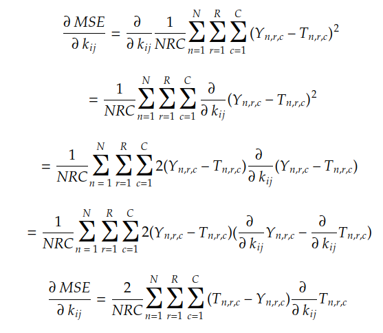
Since the values of N, R, C, Yₙ, and Tₙ are known, everything we need to calculate is the partial derivative of each coefficient in Tₙ with respect to coefficient kᵢⱼ. In the case of convolutions with padding P, this derivative is given by:

If we unroll the summations for r and c, we can find that the gradient is simply given by:

where δₙ is the matrix:

The following code implements this operation:

auto gradient = [](const std::vector<Matrix> &xs, std::vector<Matrix> &ys, std::vector<Matrix> &ts, const int padding)
{
 const int N = xs.size();
 const int R = xs[0].rows();
 const int C = xs[0].cols();

 const int result_rows = xs[0].rows() - ys[0].rows() + 2 * padding + 1;
 const int result_cols = xs[0].cols() - ys[0].cols() + 2 * padding + 1;
 Matrix result = Matrix::Zero(result_rows, result_cols);
 
 for (int n = 0; n < N; ++n) {
 const auto &X = xs[n];
 const auto &Y = ys[n];
 const auto &T = ts[n];

 Matrix delta = T - Y;
 Matrix update = Convolution2D(X, delta, padding);
 result = result + update;
 }

 result *= 2.0/(R * C);

 return result;
};

Now we know how to obtain the gradients, let’s implement the gradient descent algorithm.

Coding Gradient Descent

Finally, the code of our gradient descent is here:

auto gradient_descent = [](Matrix &kernel, Dataset &dataset, const double learning_rate, const int MAX_EPOCHS)
{
 std::vector<double> losses; losses.reserve(MAX_EPOCHS);

 const int padding = kernel.rows() / 2;
 const int N = dataset.size();

 std::vector<Matrix> xs; xs.reserve(N);
 std::vector<Matrix> ys; ys.reserve(N);
 std::vector<Matrix> ts; ts.reserve(N);

 int epoch = 0;
 while (epoch < MAX_EPOCHS)
 {
 xs.clear(); ys.clear(); ts.clear();

 for (auto &instance : dataset) {
 const auto & X = instance.first;
 const auto & Y = instance.second;
 const auto T = Convolution2D(X, kernel, padding);
 xs.push_back(X);
 ys.push_back(Y);
 ts.push_back(T);
 }

 losses.push_back(MSE(ys, ts));

 auto grad = gradient(xs, ys, ts, padding);
 auto update = grad * learning_rate;
 kernel -= update;

 epoch++;
 }

 return losses;
};

This is the base code. We can improve it in several ways, for example:

• using the loss of each instance to update the kernel. This is called Stochastic Gradient Descent (SGD), which is very useful in real-world scenarios;
• grouping instances in batches and updating the kernel after each batch, which is called Minibatch;
• Using a Learning Rate Schedule to decrease the learning rate over the epochs;
• In the line kernel -= update; we can hook up an optimizer such as Momentum, RMSProp, or Adam. We will discuss optimizers in forthcoming stories;
• Introducing a Validation Set or using some Cross-Validation Schema;
• Replacing the nestedfor(auto &instance: dataset) loop to gain performance and CPU usage by Vectorization (as discussed in the previous story);
• Adding callbacks and hooks to easier customize our train loop.

We can forget these improvements for a while. Now, the point is to understand how gradients are used to update the parameters (in our case, the kernel). This is the fundamental, core, concept in today’s machine learning and also a key factor to move forward on more advanced topics.

Let’s see how this code work by putting it into action with an illustrative experiment.

Practical Experiment: Restoring the Sobel’s edge detector

In the last story, we learned that we can apply a Sobel filter Gx to detect vertical edges:

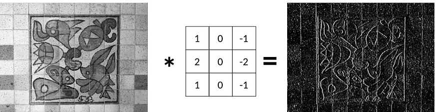
Now, the question is: given the original and the edge image, do we manage to restore the Sobel filter Gx?

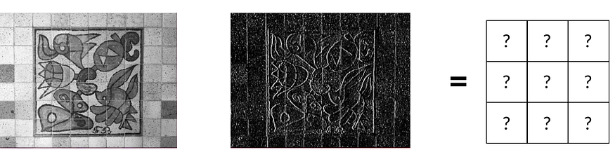
In other words, can we fit the kernel given the input X and the expected output Y?

The answer is yes and we will use the gradient descent to do that.

Loading & preparing the data

First, we use OpenCV to read some images from a folder. We apply the Gx filter on them and store them in pairs in our Dataset object:

auto load_dataset = [](std::string data_folder, const int padding) {

 Dataset dataset;
 std::vector<std::string> files;
 for (const auto & entry : fs::directory_iterator(data_folder)) {

 Mat image = cv::imread(data_folder + entry.path().c_str(), cv::IMREAD_GRAYSCALE);
 Mat formatted_image = resize_image(image, 640, 640);

 Matrix X;
 cv::cv2eigen(formatted_image, X);
 X /= 255.;

 auto Y = Convolution2D(X, Sobel.Gx, padding);

 auto pair = std::make_pair(X, Y);
 dataset.push_back(pair);
 }

 return dataset;
};

auto dataset = load_dataset("../images/");

We are formatting each input image to fit a 640×640 grid using a helper utility resize_image.

As the images above show, resize_image centralizes each image into a black 640×640 grid without stretching the image by simply resizing it.

We used the Gx filter to generate the ground-truth output Y for each image. Now, we can forget this filter. We will restore it from the data using gradient descent and 2D convolution.

Running the experiment

By joining all the pieces, we can finally see the training execution:

int main() {
 const int padding = 1;
 auto dataset = load_dataset("../images/", padding);

 const int MAX_EPOCHS = 1000;
 const double learning_rate = 0.1;
 auto history = gradient_descent(kernel, dataset, learning_rate, MAX_EPOCHS);
 
 std::cout << "Original kernel is:\n\n" << std::fixed << std::setprecision(2) << Sobel.Gx << "\n\n";
 std::cout << "Trained kernel is:\n\n" << std::fixed << std::setprecision(2) << kernel << "\n\n";

 plot_performance(history);

 return 0;
}

The following sequence illustrates the fitting process:

In the beginning, the kernel is filled with random numbers. Because of this, in the first epochs, the output image is usually a black output.

After a few epochs, however, gradient descent begins to fit the kernel toward the global minima.

Finally, in the last epochs, the output is almost equal to the ground truth. At this moment, the loss value asymptotically moves to the lowest value. Let’s check the loss performance over the epochs:

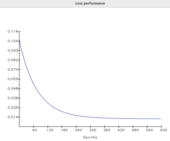
In machine learning, this loss curve shape is very common. It turns out that, in the first epochs, the parameters are basically random values. This causes the initial loss to be high:

In the last epochs, gradient descent has finally performed its work, fitting the kernel to suitable values, which makes the loss converge toward the minima.

We can now compare the learned kernel against the original Gx Sobel’s filter:

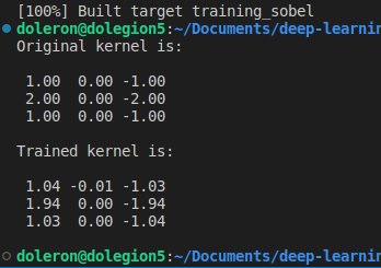
As we expected, the learned and original kernels are very close. Note that this difference can still be smaller if we train the kernel during more epochs (and use a smaller learning rate).

The code for training this kernel can be found in this repository.

A last word about differentiation and autodiff

In this story, we used common calculus rules to find the MSE partial derivatives. In some cases, however, finding an algebraic derivative for a given complex cost function can be challenging. Fortunately, modern machine learning frameworks provide a magic feature called automatic differentiation or simply autodiff.

autodiff tracks each elementary arithmetic operation (like additions or multiplications) applying the chain rule to them to find the partial derivatives. Thus, when using autodiff, we needn’t calculate the algebraic formulas of the partial derivatives or even implement them directly.

Since here we are using simple, well-known, cost formulas, making use of autodiff or even solving complex differentiation by hand is not required.

Covering derivatives, partial derivatives, and auto differenciation in more details deserves a new story!

Conclusion and next steps

In this story, we learned how gradients are used to fit kernels from data. We covered gradient descent which is simple, powerful and a base to derive more complex algorithms such as backpropagation. We also performed a practical experiment using gradient descent to restore a Sobel filter from data.

In the next story, we will cover activation functions, the different types, and the motivation behind using them. We will learn how to code them and how to code their derivatives.

Reference Books

Machine Learning, Mitchell

Cálculo 3, Geraldo Ávila (in Brazilian Portuguese)

Neural Networks: A Comprehensive Foundation, Haykin

Pattern Classification, Duda

Computer Vision: Algorithms and Applications, Szeliski.

Python machine learning, Raschka

Join thousands of data leaders on the AI newsletter. Join over 80,000 subscribers and keep up to date with the latest developments in AI. From research to projects and ideas. If you are building an AI startup, an AI-related product, or a service, we invite you to consider becoming a sponsor.

Published via Towards AI