


Classification Metrics Clearly Explained!
Last Updated on July 25, 2023 by Editorial Team
Author(s): Jose D. Hernandez-Betancur
Originally published on Towards AI.
Let’s dive into the classification metrics
1. Introduction
One of the first things that people who are new to data science learn is how to measure how well algorithms work. When I first started learning about data science, I thought that the people who made the courses thought that introducing the metrics and their equations was more than enough to choose a good measure and train a high-performance model. This way of teaching couldn’t be further from the truth U+1F3DC️. Each measure has a practical explanation that should be looked into, especially when you consider what could happen if you don’t choose the right classification metric. These metrics are part of the basic tools that any data scientist should have, and not just for a job interview.
Drawings and colors were one thing that helped me understand some things during my BS. So, I’ll try to explain classification metrics in this way, especially to people who are new to the area of data science. So, join me if you are new to the field or want to find a new way to explain these metrics. Let’s push the limits of what we know and how we know it U+1F91CU+1F9F1U+1F680…
2. What Do Metrics Mean?
2.1. TP, TN, FP, FN, and Consufion Matrix
Before explaining the metrics, let’s go over some terms that are mandatory to understand. A classification problem is like the hypothesis tests widely used in inferential statistics (in fact, in machine learning, we assume a shape for the real data's statistical distribution, i.e., we use a surrogate model). Thus, we can draw a parallel with hypothesis testing.
Generative models vs Discriminative models for Deep Learning.
Get expert insights into generative and discriminative models, and find out which of the two is best suited for deep…
www.turing.com
You are a data scientist working for a hospital. The hospital requires you to build a classifier to predict whether patient is healthy or sick. Thus, the trivial or null hypothesis is that patience is healthy, while the research or alternative hypothesis is that patience is sick. Labels in favor of H₀ (or the null hypothesis) are called negative, no matter if they actually are, while labels in favor of Hₐ (or the alternative hypothesis) are named positive, regardless of whether they are true.
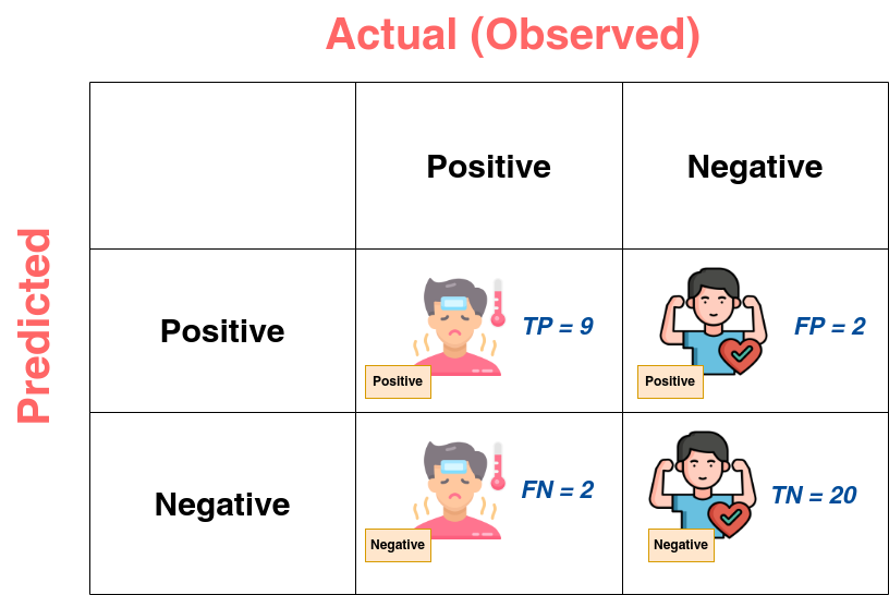
Thus, after training the classifier, you get a figure such as the one presented in Figure 1. The person shapes serve as a representation of the actual target value for labeled data, whereas the tags are the classifier's predictions after obtaining the decision boundary through training.

- True Positive (TP): TP is the case when positive labels predicted by the classifier agree with reality. In Figure 1, TP is when a positive tag accompanies a sick man. Here, TP equals 9.

- True Negative (TN): TN is the case when negative labels predicted by the classifier agree with reality. In Figure 1, TN is when a negative tag accompanies a healthy man. Here, TN equals 20.

- False Positive (FP): FP is the case when positive labels predicted by the classifier disagree with reality. In Figure 1, FP is when a positive tag accompanies a healthy man. Here, FP equals 2.

- False Negative (FN): FN is the case when negative labels predicted by the classifier disagree with reality. In Figure 1, FN is when a negative tag accompanies a sick man. Here, FN equals 2.

- Confusion Matrix: The confusion matrix, also called the confusion table, is a way to describe the results of the classification or to bring together TP, TN, FP, and FN. Most of the time, the true (or observed) value is in the columns, and the predicted value is in the rows.
Although the above terms are explained with binary problems, they are extendable to multi-class (mutually exclusive classes) and multi-label (no mutually exclusive classes) classification problems.
2.2. Classification Metrics
Now, let’s explain the classification metrics, considering the above example.
- Accuracy: Accuracy is the most intuitive classification metric. Thus, I won’t extend a lot of the discussion in this part. The accuracy is the ratio between the correctly predicted labels and the total or existing labels.

- Recall: The recall metric is also known as the sensitivity or true positive ratio (TPR). In simple words, this is the ability of a classifier to correctly classify the actual total positive labels as positive.

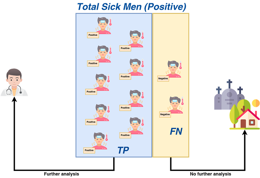
As Figure 7 shows, recall is a metric that focuses on all existing positives. If the classifier is like triage in a hospital, a high-recall model will send almost all of the people who are really sick to the doctor for more study.
- Specificity: The specificity is also known as the true negative ratio (TNR). In simple words, this is the ability of a classifier to correctly classify the actual negative labels as negative.

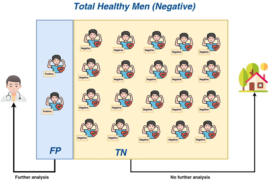
As Figure 8 shows, specificity is a metric that focuses on all the negatives that already exist. If the classifier is set up as clinical triage, a high-specificity model will send almost all of the healthy people back to their homes.
- Precision: This metric is the ratio between the true positives (TP) and the total samples predicted as positive by the classifier.

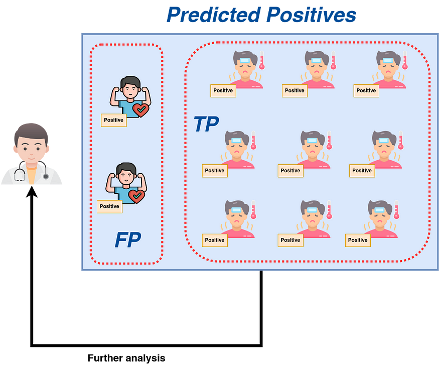
Even though precision, like recall, focuses on positives, it does so by paying attention to positive labels that were predicted. If a model is high-precision, it will make sure that most of the people sent from triage to the doctor for further testing are truly sick (see Figure 9).
- F1 Score: As we’ll see later, there’s a trade-off between recall and precision. So, the F1 Score is used to keep this balance in check. The harmonic mean of recall and precision is used to figure out F1. The F1 Score could also be seen as a balance between FP and FN.

Though the examples are for binary classification, the foundation holds true for multi-class and multi-label problems. Explore micro, macro, and weighted averages.
3. What Metric Should I Select?
Based on the goal of each metric, you can build a “decision tree” that shows the steps you need to take to choose the right metric for your classification problem. Figure 10 depicts a decision tree for classification metrics. Use this as a guide or starting point, and don’t forget to dig deeper into the rules that are important for your machine learning system.
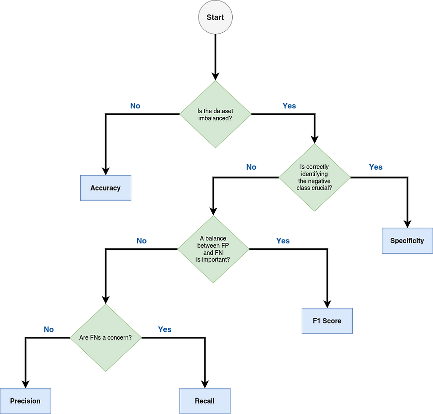
In the above tree, the first split node considers whether the dataset is imbalanced. An imbalanced dataset is one where the samples for each class are considerably different. To explore this topic and alternatives for solving this problem, check the materials below U+1F447…
5 Techniques to Handle Imbalanced Data For a Classification Problem
Techniques to handle imbalanced data for a classification problem. Here we discuss what is imbalanced data, and how to…
www.analyticsvidhya.com
imbalanced-learn documentation – Version 0.10.1
The user guide provides in-depth information on the key concepts of imbalanced-learn with useful background information…
imbalanced-learn.org
- Accuracy: As the decision tree shows, accuracy is adequate when the dataset is balanced or you apply any strategy to balance the classes.
- Specificity: As shown in Figure 10, when you are more worried about properly identifying whether something belongs to the negative class, specificity is the metric to choose. The example presented in Figure 8 is not adequate to illustrate the benefits of using specificity U+1F644. But I promised a good explanation U+1F60E.
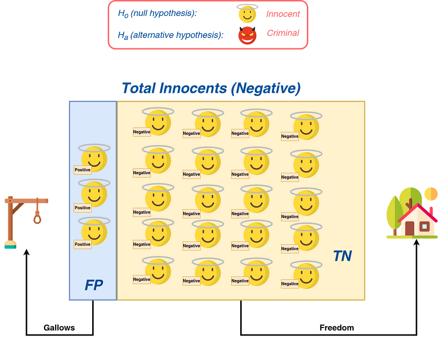
So, let’s say you have a model that needs to figure out if someone is innocent or guilty. If the person is innocent, he will be set free. If he is guilty, he will be hanged (see Figure 11). Thus, in this case, it is better to use a model with as much specificity as possible because a mistaken model can send an innocent to the gallows (and he never came back U+1F614).
- F1 Score: This metric is normally used in cases of imbalanced learning. As mentioned in the decision tree in Figure 10, this metric is not only adequate when predicting the positive class properly, which is important, but also when it is important to find a balance between recall and precision, or as the same, between the FN and FP (see the equations for recall and precision).
- Recall: This metric is good enough when the goal is to correctly classify the positive group and lower the chance of FNs. One good example is Figure 7. No decrease in FNs can lead to sick people being sent home without treatment, like chemotherapy for cancer.
- Precision: This metric is good when you want to predict the positive class and reduce the chance of FPs. Figure 12 shows a situation in which you are looking into possible items to make and put on the market. If your classifier suggests the product will be profitable, you will spend money on its manufacture, advertising, and distribution. So, the risk of FPs will go down or go away if the precision is close to one.
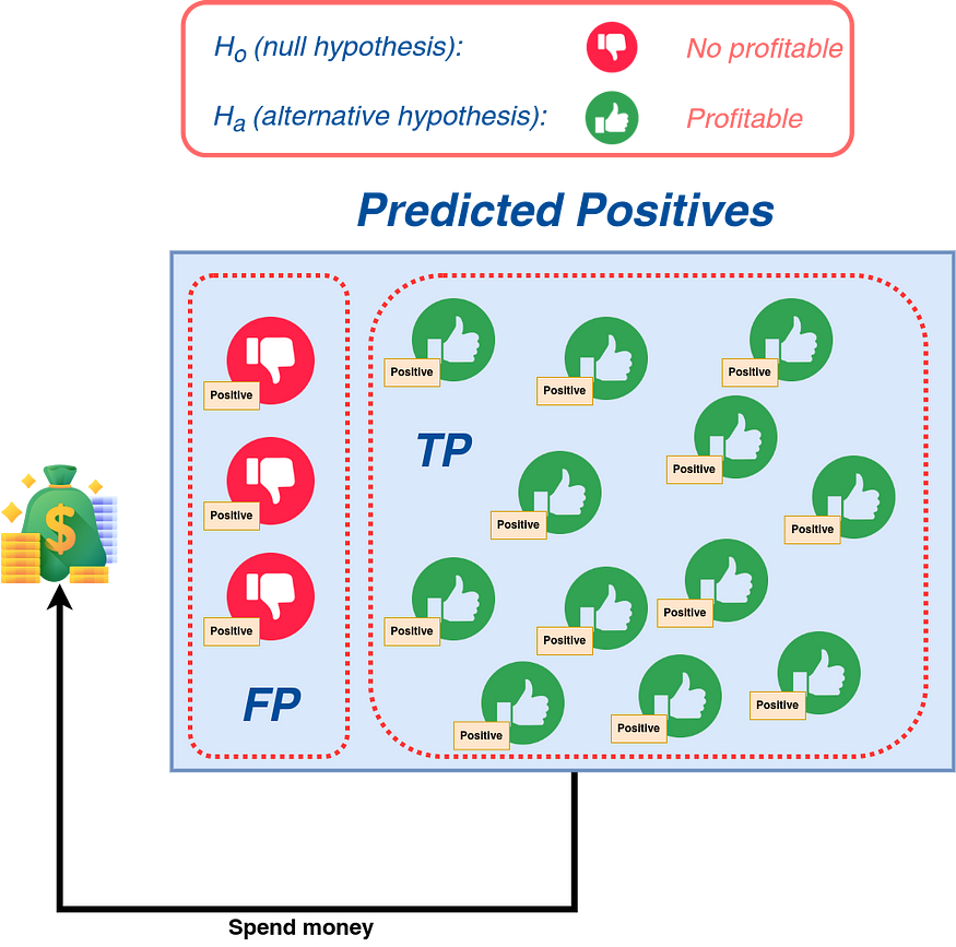
Think about the worst-case and best-case scenarios. Both are important, or one is more important than the other?
4. What About the Classification Threshold?
In classification, we use a threshold to define whether a prediction lies on the side of the positives or negatives. The selection of this threshold has implications for the classification metrics.
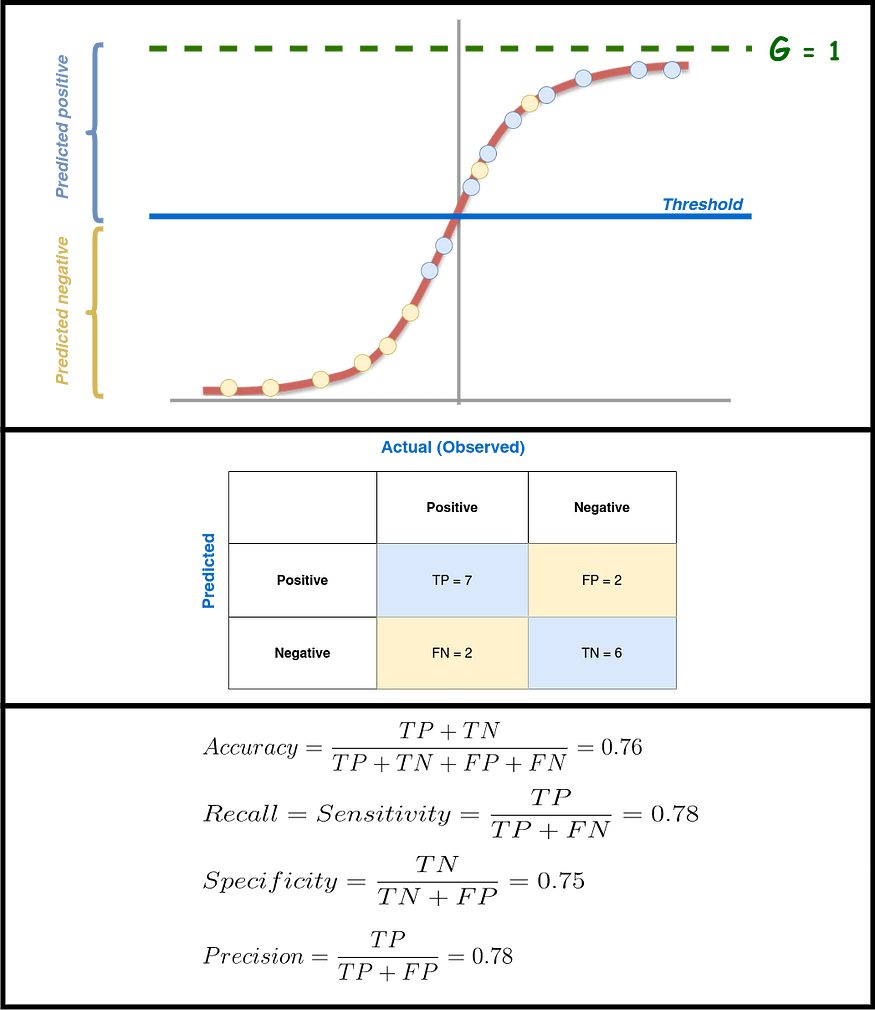
Figure 13 shows an example of applying a sigmoid function to an output to obtain values between 0 and 1. In Figure 13, the threshold equals 0.5, which is the value normally used. Figure 13 shows the confusion matrix for this case and the values of accuracy, recall, specificity, and precision.
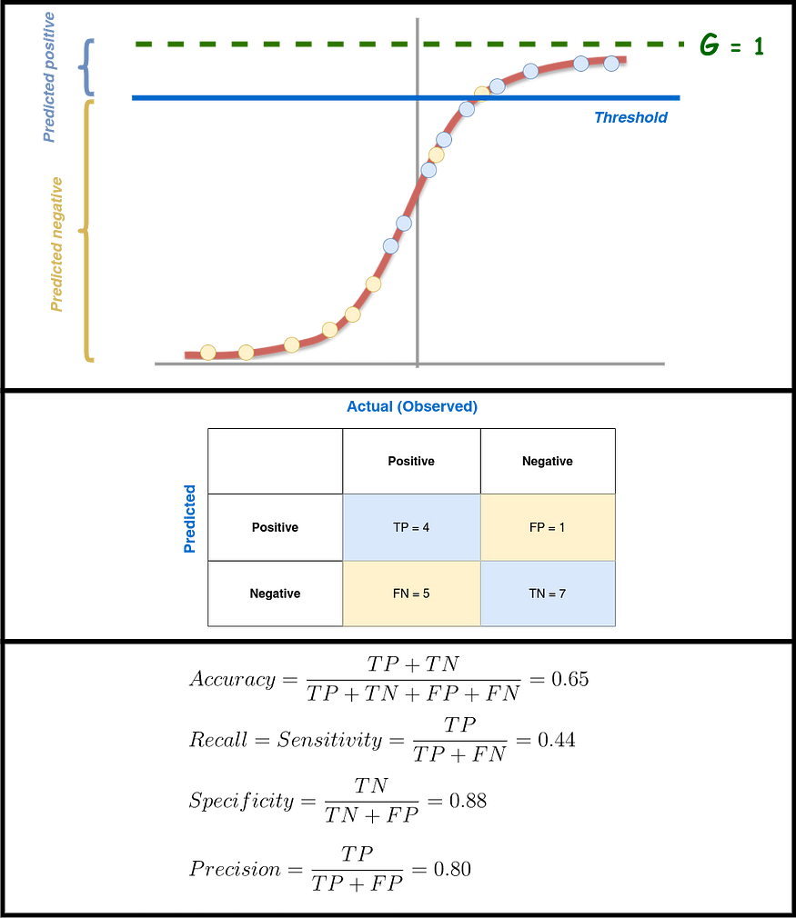
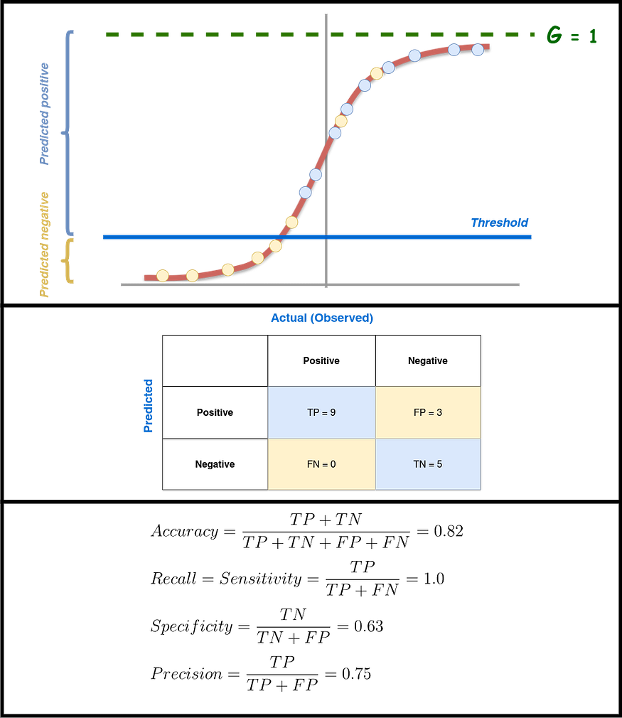
If the threshold number is raised, the FNs go up and the FPs go down. This means that recall goes down and precision goes up. This is shown in Figure 14, where the threshold gets closer and closer to 1. This shows the FN-FP trade-off, also called the Recall-Precision trade-off. If, on the other hand, the threshold gets closer to zero or goes down, FNs go down while FPs go up (see Figure 15). This means that recall goes up while precision goes down. So, when making a classifier, you should choose the right threshold by thinking about what each metric means and how well the model performs based on the rules your machine-learning system should follow. For the above, using the receiver operating characteristic curve, or ROC curve, can help you in this endeavor (see below U+1F447).
Classification: ROC Curve and AUC U+007C Machine Learning U+007C Google for Developers
Estimated Time: 8 minutes An ROC curve ( receiver operating characteristic curve) is a graph showing the performance of…
developers.google.com
Conclusions
In this post, we looked at important terms for classification learning, such as false positive (FP), false negative (FN), true positive (TP), true negative (TN), and confusion matrix. We look at the meaning of the most popular classification metrics, such as accuracy, recall, specificity, precision, and F1 Score, by showing them in pictures. We looked at situations where each metric was better and more hopeful than the others. We also looked at what it means to use different thresholds in the classification models and how they play a big role in the trade-off between recall and precision.
If you enjoy my posts, follow me on Medium to stay tuned for more thought-provoking content, clap this publication U+1F44F, and share this material with your colleagues U+1F680…
Get an email whenever Jose D. Hernandez-Betancur publishes.
Get an email whenever Jose D. Hernandez-Betancur publishes. Connect with Jose if you enjoy the content he creates! U+1F680…
medium.com

Join thousands of data leaders on the AI newsletter. Join over 80,000 subscribers and keep up to date with the latest developments in AI. From research to projects and ideas. If you are building an AI startup, an AI-related product, or a service, we invite you to consider becoming a sponsor.
Published via Towards AI
Related posts


Popular posts

 for 2021")


Updates

Recent Posts


