YOLOV5(m): Implementation From Scratch With PyTorch

Author(s): Alessandro Mondin

Originally published on Towards AI.

The prerequisites to understand this article are a good understanding of PyTorch and a basic comprehension of YOLO architectures.

U+26A0️ Since You Only Live Once, think twice before implementing a YOLO algorithm from scratch. It might hurt your mental health.

Important assumptions:

• You should not read this article if you are looking for an in-depth explanation of Ultralytics’ autoanchor algorithm since I am giving a high-level description.
• I am writing this article on December 2022, and the version of YOLOv5 that I am going to describe is YOLOv5 v6.0. In fact, YOLOv5 shouldn’t be considered an algorithm but an object detection and segmentation repository that is continuously updated and improved (the algorithm, the augmentations, loss functions, etc.).

Among all the files present in my YOLOV5 GitHub repo, in this article, I am focusing on model.py. Let’s start!

Note: as of today the indentation of long Gists is broken, if you face this problem click on “view raw”!

Considering that YOLOv5 isn’t published in any Arxiv paper (as of December 2022), the information available online is scattered and often not up-to-date with the latest releases.

After a lot of research, the best visualization that I’ve found is the following:

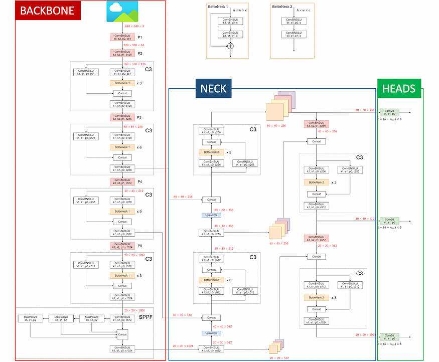
Firstly, what arises from this visualization is that, as with all YOLO algorithms, the architecture can be conceptually separated into three chunks:

1. The backbone, whose task is to extract deep-level features (feature-extractor).
2. The neck combines information from layers of different depths (feature aggregator).
3. The heads are responsible for the predictions.

Secondly, the image shows that most of the architecture is composed of the repetition of a few convolutional blocks:

• C3
• Bottlenecks
• SPPF

“But where can I find the details on each layer?”

After some research, I identified two ways:

1. Read Ultralytics .yaml files and, with the help of the visualization above, attempt to translate the blocks into PyTorch classes.
2. Export the model to .onnx format and visualize it on Netron.

The first approach seemed too complex and mechanical since .yaml files are understandable once you’ve already comprehended YOLOv5 architecture. Therefore I opted to use Netron.

I exported YOLOv5 to .onnx format with Ultralytics export.py, and then I uploaded the the .onnx file on Netron, which is a tool that “translates” the model architecture into an easy-to-follow visualization.

Here below, YOLOv5(m) input and output layers visualized with Netron.

At this point, I started translating the visualization into PyTorch.

The first step was creating a CBL class that is used throughout the whole architecture:

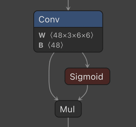
But why SiLU? The answer is experiments. They started with ReLU, then LeakyReLU, then ….. SiLU.

Backbone

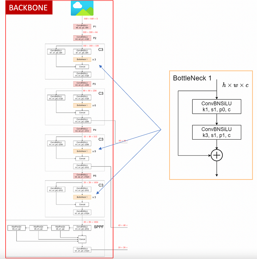
As shown in the images, the backbone is composed of the following CNN blocks:

• ConvBNSiLU (the CBL defined above)
• BottleNeck 1
• C3
• SPPF

BottleNeck 1 is used to build the C3 block (it’s embedded), so let’s start with it.

Bottleneck 1 is a residual block with two skipped connections that, besides improving gradient back-propagation, comes with a width_multiple parameter. This parameter, usually referred to as the expansion factor, controls how much we want to squeeze and re-expand the number of channels between c1 and c2 . This logic of squeezing & expanding channels was initially introduced by this paper.

Once define the Bottleneck, I’ve created the C3 class which is the bulk of YOLOv5 backbone.

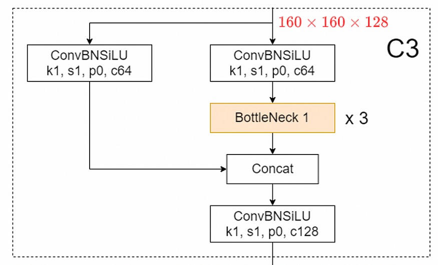
The C3 block is a simplified variant of CSP blocks, which was created to increase the diversity of back-propagated gradients.

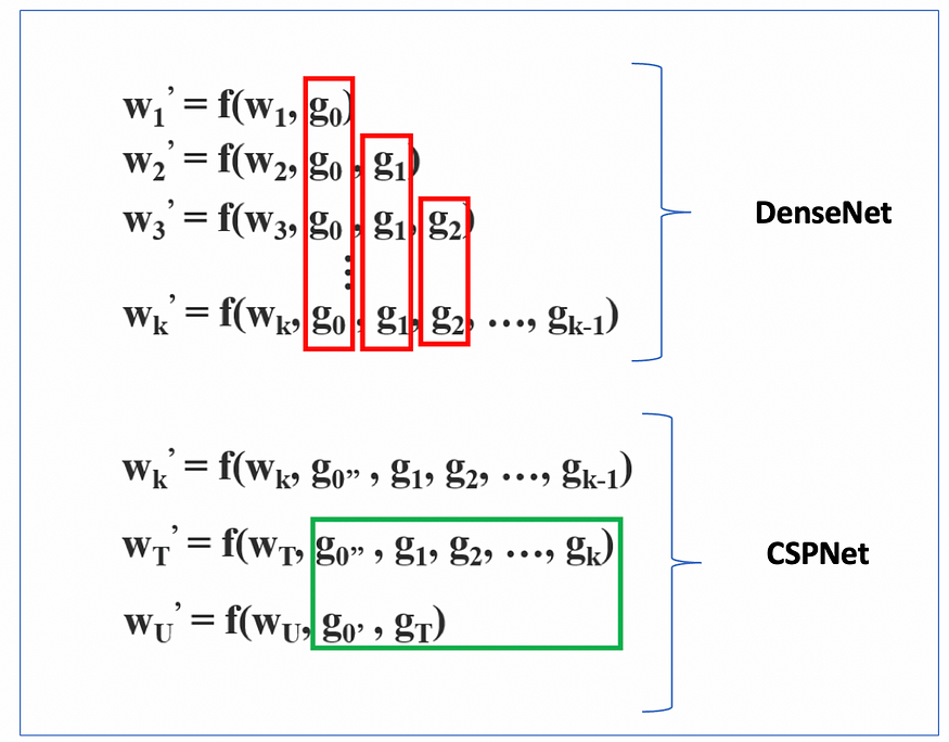
In fact, the gradients flowing backward with a CSPNet-style block are less duplicated compared to the ones of a DenseNet (image above) , which translates into better results.

I invite you to check the code above. Anyway, the aspects that need to be highlighted are:

• The presence of the width_multiple (expansion factor).
• A depth parameter that controls the number of sequential repetitions of the Bottleneck blocks.
• The output of the sequence of “Bottleneck 1” blocks and the output of the skipped connection are concatenated channels-wise (along dim=1), and the resulting tensor is fed into the last convolution c_out (check the forward method).

The last CNN block used to build the backbone is the SPPF (Spatial Pyramid Pooling Fast) which is a faster variant of the SPP layer introduced in 2015.

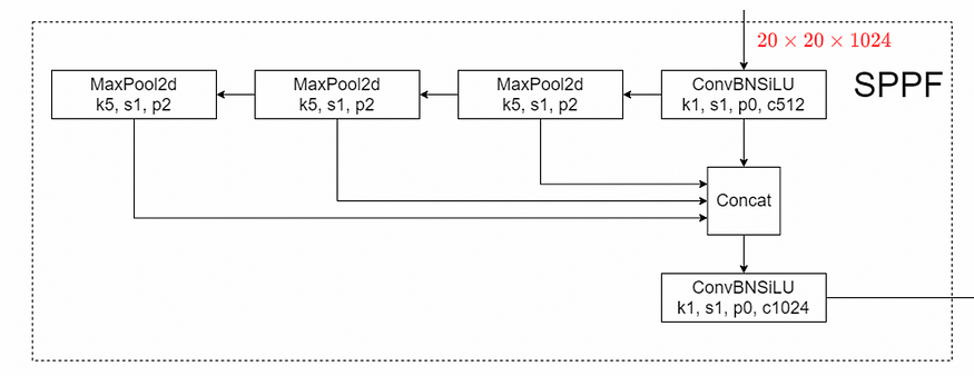
Although the original purpose of an SPP was to create a fixed-size vector from any input size, after testing Ultralytics SPPF, I noticed that this behavior couldn’t be replicated (others noticed it too). However, as the YOLOv5 creator replied in the link here above, SPPF is mathematically identical to the original SPP layer but faster.

Therefore, I summed up that in YOLO architectures, SPP layers are not used for their initial purpose (fixed-size output), but instead, they’re used to exploit their functionality of feature re-aggregators achieved through sequences of max pooling and concat.

Since we have completed all the distinct blocks that compose the backbone we can just put them together to create the YOLOV5 backbone.

Neck

Yolov5 neck is PANet style (Path Aggregation Network).

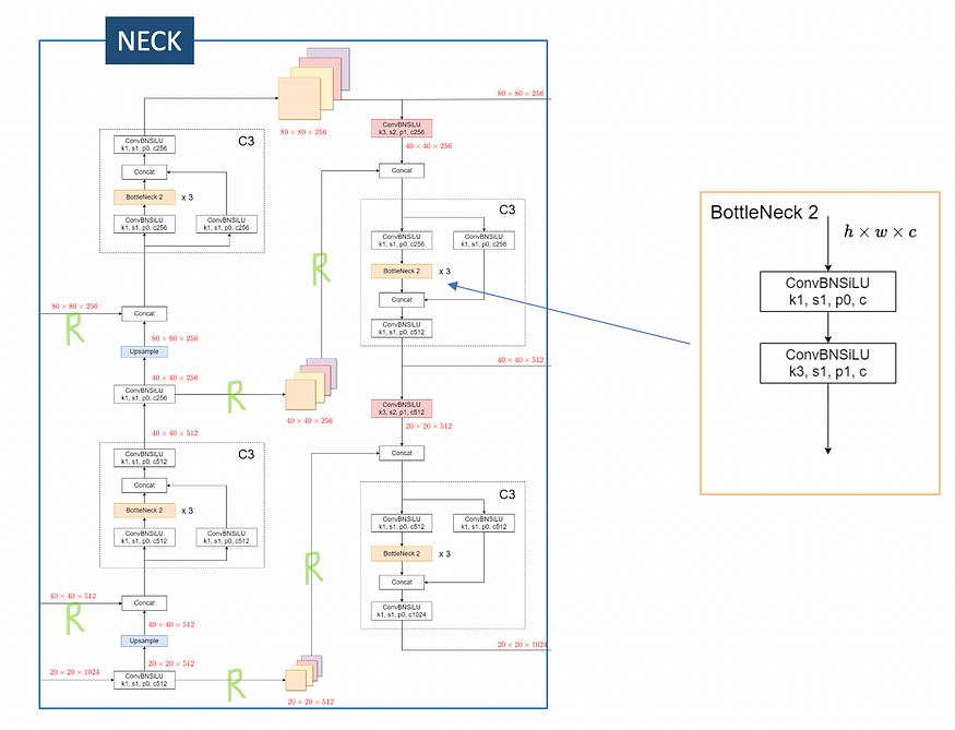
PANet stands for “Path Aggregation Network” and its core functionality is to enhance the flow of information between the lower layers and topmost features via route connections, marked in the image above with “R”. If you look at the image above, in fact you can notice:

• Features from different depths of the backbone that are combined (concatenated) into the neck (the two “R” in the left).
• Features from the beginning of the neck are concatenated with features in the last part of the neck that precede the heads (the four “R” in the middle)

In terms of CNN blocks, the neck is composed by these operations:

• ConvBNSiLU
• BottleNeck 2
• C3
• Upsample
• Concat

As you remember, in the backbone, inside the C3 blocks, we were using “bottleneck 1” which is characterized by the skipped connection. The “bottleneck 2”, on the other hand, it’s just a sequence of two convolutions (lines 31 and 32 below).

The C3 class is the same used in the backbone previously, with the difference that here we are setting the C3's parameter backbone=False.

So by putting the pieces together, we create the neck.

While Ultralytics YOLOv5 uses nn.Upsample and nn.Concat (to facilitate versioning via .yaml files), in my implementation, I’ve used torch.nn.functional, and therefore, upsampling and concatenation are performed in the forward method.

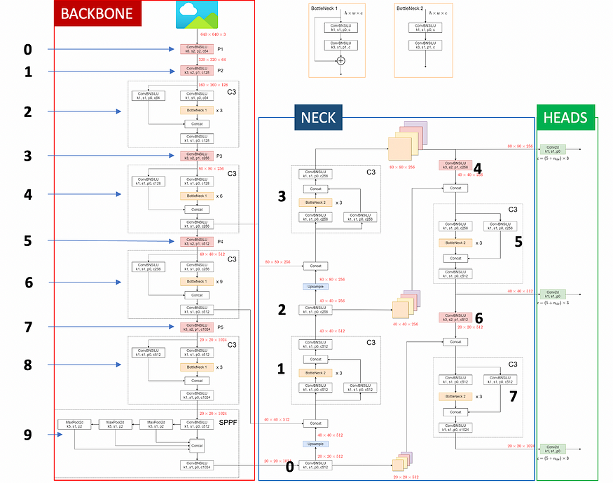
In this image of the YOLOv5 architecture, I marked the position (idx) of the distinct blocks inside self.backbone and self.neck.

In my YOLOV5 forward() shown below, you can notice that:

• If a backbone layer is a C3 and the idx is 4 or 6, we append the output to a list used to store backbone route connections.
• If a neck layer has idx 0 or 2, we store the output to a list containing neck route connections, then we resize the tensor (same as Upsample), and concatenate it with the last element of the backbone route connections (that is deleted with .pop() ).
• If a neck layer has idx 4 or 6, the output layer is concatenated with the last element of the neck route connections (that is deleted with .pop() ).
• Lastly, If a neck layer is C3 and the idx is greater than 2, we store the output tensor to a list that will be then fed to the model heads to perform a prediction.

The last step is to define YOLOv5 heads.

Heads

If you’re not already familiar with YOLO heads and you’re already struggling to understand what explained up to now, I encourage you to take a break because heads are by far the most complex part of the architecture

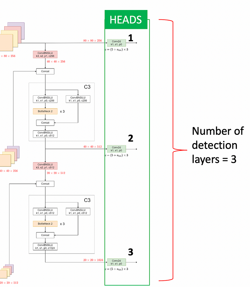
To understand YOLO(v5) heads, we need to clarify these key concepts:

1. Grid-cells
2. Detection layers
3. Predictions per scale
4. Anchor boxes
5. From grid cells to bounding boxes

1. Grid-cells

YOLO algorithms provide the localization of objects through coordinates expressed w.r.t. the center of a grid-cell.

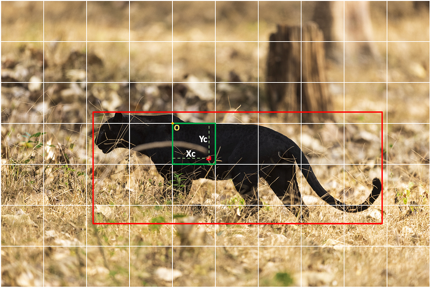
Remind: in YOLO algorithms each grid-cell can detect at most one object.

The image above, for example, contains a 7 x 10 grid-cells (hxw), and the one responsible for detecting the panther is highlighted in green.

Each grid-cell is a vector of 5 + num_classes values which contains the following information:

1. Objectness_score which represents the likelihood of the presence of (the centre of) an object within the grid-cell.
2. Xc that represents the horizontal distance between the origin of the grid-cell (top-left) and the center of the object.
3. Yc represents the vertical distance between the origin of the grid-cell (top-left) and the center of the object.
4. Width is measured w.r.t the width of the grid-cell: considering the panther above, width is ~6.5 (details later in 2)Detection layers ) .
5. Height is measured w.r.t the height of the grid-cell: considering the panther above, height is ~ 2.5 (details later in 2)Detection layers ) .
6. Classes are a vector of len = len(n_classes) where the values represent the likelihood of an object belonging to each class.

NB: the Objectness score is crucial in YOLO algorithms. For example, in the image above, among the 70 grid_cells, only the one highlighted with green has an objectness_score > confidence_threshold, which indicates the possible presence of an object (we enforce this behavior during YOLOv5 training).

2. Detection layers

len(yolo_output) == num_detection_layers

In YOLO algorithms, a detection layer is a synonym for the head. YOLOv5 default architecture uses 3 detection layers (first image of this chapter) and each one specializes in detecting objects of a given size. Precisely:

• the head 1 (80 x 80 grid cells) is suitable for detecting small objects
• the head 2 (40 x 40 grid cells) is suitable for detecting medium-sized objects
• the head 3 (20 x 20 grid cells) is suitable for detecting large objects

The reason why each layer is suitable for detecting certain object-sizes is related to grid-cells: for example, considering that each cell can detect at most one object, the upper grid could detect at most 4 sheep, while the second one up to 64 sheep.

Another crucial aspect is that for each detection layer, the outputted grid is composed of grid-cells that represent a certain width and height of the original image:

1. The first detection layer outputs a grid where each grid cell represents a width and a height of 8 pixels of the original input image (80×8 = 640).
2. The second detection layer outputs a grid where each grid_cell represents a width and a height of 16 pixels of the original input image (40×16 = 640).
3. The third detection layer outputs a grid where each grid_cell represents a width and a height of 32 pixels of the original input image (20×32 = 640).

80×80, 40×40 and 20×20 is the size of grid_cell assuming an input image of [3, 640, 640]

N.B: the width and height represented by grid cells are scale-invariant: if the input size increases, in turn, the dimension of the output grid increases, but the pixels expressed by each grid_cell are always going to be 8, 16, and 32.

In YOLOv5, [8, 16, 32] are referred as the “strides” of the model.

3. Predictions per scale

Each detection layer ~ head is, in turn, specialised to detect different sub-scales (aspect-ratios), by default 3.

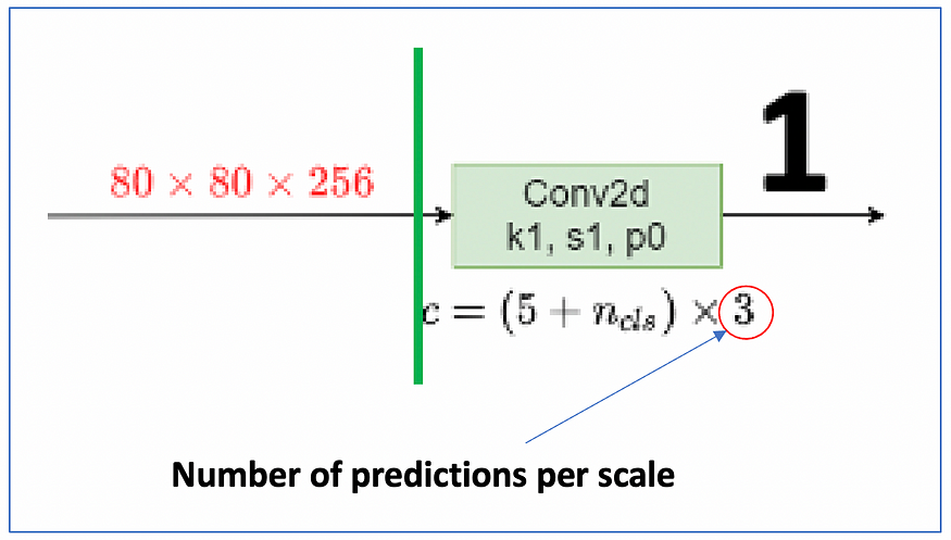
For example, the first detection-layer shown here will specialize at detecting 3 different sub-scales of small objects, such as

1. small rectangular-horizontal objects
2. small squared objects
3. small rectangular-vertical objects

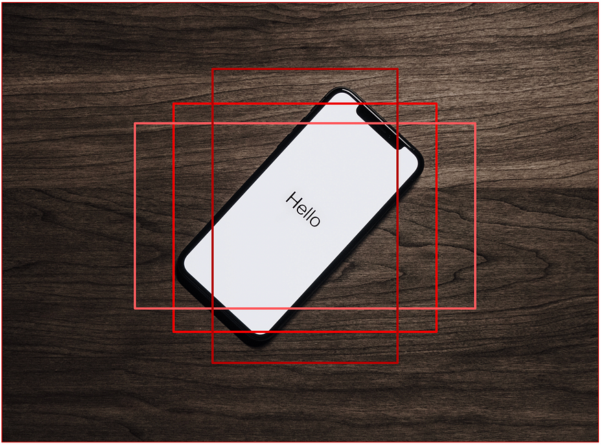
NB: These three aspect-ratios (rect-vertical, squared and rect-horiz) are just an example. They depend entirely on the dataset and, in YOLOv5, are identified through the “autoanchor algorithm”. Details in 4) Anchors.

To summarise what explained up to this point:

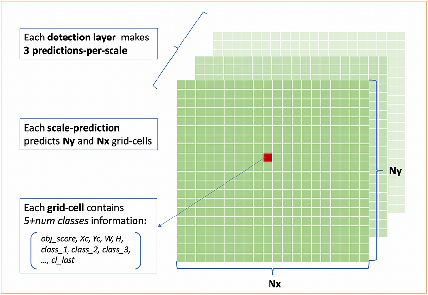
Therefore, by feeding a [3, 640, 640] image to a default YOLOV5m (3 detection-layers and 3 predictions-per-scale), the amount of grid-cells predicted is:

tot_grid_cells = (3 x 80 x 80) + (3 x 40 x 40) + (3 x 20 x 20) = 25200

4. Anchor Boxes

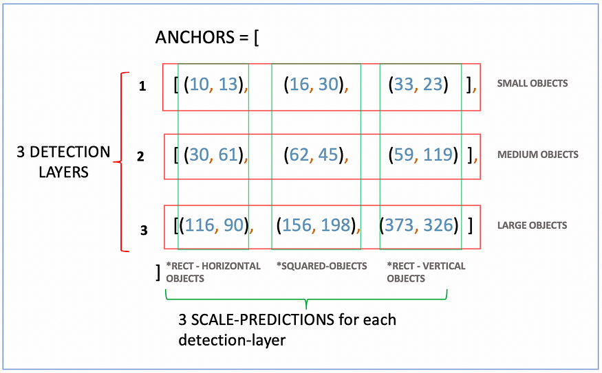
An anchor-box is a couple of 2 integers that indicate width and height expressed in pixels. In some cases, you can find it expressed with floats [0, 1] and represent W_box/default_image_size and H_box/default_image_size

(10, 13) means 10 pixels of width and 13 pixels of height

Anchor boxes (also referred to as anchors) are obtained by running K-Means clustering across the object labels, and the resulting K-centroids represent the main aspect-ratios (W, H) of the objects of the target datasets. Since a default YOLOv5 architecture has 3 detection layers and 3 predictions per scale, the standard number of anchors is 9.

Practical example. Consider:

– a dataset composed by 1000 images and 1 object per image.

-1000 object labels in YOLO format (class_idx, Xc, Yc, W, H)

– a default YOLOv5 model (3 heads and 3 scale-predictions per head) → 9 anchors

We subset all the object labels and we consider only [W, H] because we are interested only on the aspect-ratios of the objects and not on their location within images. On our [1000, 2] dataset, we run K-Means with n_centroids=9. The resulting 9 centroids are 9 couples of (W, H) that represent the average width and height of each scale.

Besides K-Means, Ultralytics adopts further techniques to compute anchors through the autoanchor algorithm. Glen Josher, YOLOv5 creator, explains that autoanchor “uses kmeans centroids as initial conditions for a Genetic Evolution (GE) algorithm. The GE algorithm will evolve all anchors for 1000 generations under default settings, using CIoU loss (same regression loss used during training) combined with Best Possible Recall (BPR) as its fitness function.” U+1FAE0

Despite describing autoanchor is not in the scope of this article, if you run it before training your YOLOv5 on a custom dataset, you’ll make sure that the default MS COCO anchors (in the image below) correctly suit the objects present in your dataset. If MS COCO anchor don’t suit your objects, autoanchor will suggest you an alternative set of anchors.

Last but not least, in YOLOv5 anchors are not updated during training. As explained here, they noticed empirically that making anchors learnable parameters didn’t improve the results.

As Aladdin Persson brightly says:

Using Anchor boxes is way to encode previous knowledge into the model before starting the training process

In other words, before the training process, we are already telling the model which is the (average) aspect-ratios of the objects that it has to detect. The great advantage of using anchor-boxes is that they tremendously reduce the amount of training data necessary to obtain good detections.

Good! We have defined what anchors are and how they are computed. But how do we incorporate them with the output of the model?

We achieve it by using the formulas explained in this last chapter that serves two purposes.

5) From grid cells to bounding boxes

To complete our YOLOv5, we need to solve these last two problems:

1. Integrate the output of the model with anchors
2. Transform the output coordinates from being w.r.t. grid cells to being w.r.t. the image (bounding boxes).

These two tasks, despite being related to different problems, are commonly grouped together and are solved through the formulas shown below:

As we said in the grid cells chapter: YOLOv5 predicts 25200 grid_cells when fed with a (3, 640, 640) image. Each grid_cell is a vector composed by (5 + num_classes) values where the 5 values are [objectness_score, Xc, Yc, W, H].

Bw and Bh are responsible for integrating the anchors with YOLO outputs by ensuring that when the model’s outputs W(=tw) and H(=th) are equal to 0, then default anchors, Pw and Ph are used (if an anchor is (10, 13), pw=10 and ph=13). This property is referred to as f(0)=1.

Secondly, Bx and By are responsible for translating the output of the model from being w.r.t. grid_cells to bounding boxes. Initially, by “sigmoiding” the outputs X(=tx) and Y(=ty) between 0 and 1 (coord w.r.t. grid_cells) and then by adding the grids Cx and Cy that translate the grid_cell coordinated to image coordinates.

And why YOLOv5 introduces a new formula?

According to Glen Josher, the main reason was to remove the “exponential” from the equation, which created too many downsides. In addition to that, they wanted to maintain the f(0)=1, which guarantees that for an output equal to 0, default anchors are used. That’s it!

Sooo, we have mentioned everything about YOLOv5 heads!

To summarise:

• YOLOv5 has, by default 3 detection layers specialized in detecting objects of different dimensions.
• Each detection layer makes, by default, three scale predictions, and each of these scale predictions is specialized in detecting objects of a specific aspect-ratio.
• Each scale-prediction predicts a grid of grid-cells.
• Each grid cells is composed by 5 + n_classes values which are [objectness_score, Xc, Yc, W, H, prob_class_1, .. , prob_class_n]
• The output of the model finally uses the equations explained above to incorporate anchors and to transform the output from grid_cells coordinates to bounding boxes.

Example: after feeding a (3, 640, 640) input-image to a YOLOv5 model created to detect 80 classes, the final output is a list output whose lenght is equals to len(n_detection layers). Each element of output is going to be:

output[0].shape = (batch_size, 3, 80, 80, 85)

output[1].shape = (batch_size, 3, 40, 40, 85)

output[2].shape = (batch_size, 3, 20, 20, 85)

Where 3 is n_predictions_per_scale. [80, 80], [40, 40], [20, 20] are the dimensions of the “grids of grid_cells”. 85, result of 5 + n_classes, are the values present in each grid_cell.

Let’s finally implement it with PyTorch!

To seek explainability, I’ve divided the model prediction and a function responsible for incorporating the model’s output with the above formula.

This is the YOLOv5 head class, and the forward() takes as input the output list of the YOLOv5 neck and, for each tensor-element of the list, performs a scale prediction. The details that are worth to be mentioned are:

• In line 12, register_buffer() is used to store the parameters of the model “which should be saved and restored in the state_dict, but are not trained by the optimizer”. Source here.
• Anchors are strided. In other words, for each detection layer, anchors are divided by the corresponding stride: (10, 13) is stored as (10/8, 13/8) →(1.25, 1.625)
• The CH parameters are a list that contains the number of out_channels of each element of YOLOv5 neck’s output.
• Lastly, in line 23, the reason why (5+num_classes) is set as the third dimension to be then permuted as dimension is just “legacy from YOLOv3,” as explained by Glen Josher here.

Lastly, we incorporate anchors in the output, and we transform grid cells into bounding boxes:

In my repository, this function comes with more functionalities used for experimenting. Here to seek explainability, I’m showing only the key one used for model inference.

This function takes as input the output of the YOLOv5 (heads) and performs a series of operations:

1. create the Cx and Cy grid
2. creates an anchor grid.
3. Sigmoids the whole YOLOv5 output and then applies the formula at lines 14 and 15.
4. Lastly filters the vector of classes by selecting the class that has the maximum likelihood (we select it by the index, and the value is discarded).

Let’s go in order.

1. XY_GRIDS (CX and CY)

Cx and Cy are staked together, and they are expressed by the variable xy_grid, which created a grid that looks like this one:

x_grid = torch.arange(nx)
x_grid = x_grid.repeat(ny).reshape(ny, nx)
y_grid = torch.arange(ny).unsqueeze(0)
y_grid = y_grid.T.repeat(1, nx).reshape(ny, nx)
xy_grid = torch.stack([x_grid, y_grid], dim=-1)
xy_grid = xy_grid.expand(1, naxs, ny, nx, 2)

For example, given:

• model strides of [8, 16, 32]
• a YOLOv5 output that is a list of len(n_detection_layer)
• output[0] of shape (bs, predictions_x_scale, 10, 10, 85) where 10 and 10 are the dimensions of the grid of grid cells
• 1 object is detected in (3, 2), as in the image above and its values are [obj_score=0.55, xc=0,2, yc=0.1, w=1.22, h=1.36, …n_class_prob]

By summing 3 + 0.2 (grid x coord and xc) and 2 + 0.1 (grid y coord and yc) we get (3.2, 2.1) and by multiplying it by the width of the grid cells (same as strides[0]) we get (3.2, 2.1)*8=(25.6, 16.8) which is the final center of our bounding box!

In reality, you have to compute the coordinates with YOLOv5 formulas explained previously, but the logic is the exact same.

1. ANCHOR GRID

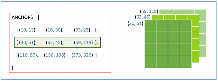
anchor_grid = (anchors[i]*stride).reshape((1, naxs, 1, 1, 2)).expand(1, naxs, ny, nx, 2)

The Anchor grid makes sure that for each detection layer, the W and H of the grid_cells ( [obj_score=0.55, xc=0,2, yc=0.1, w=1.22, h=1.36, …n_class_prob]) are multiplied for their respective anchor boxes. For example, as shown in the image, all the w and h of the grid cells in the first grid (darker one) are multiplied by 30 and 61.

Notice that since anchors are expressed relative to the width of cells (stride), we need to scale them back by multiplying them with the respective stride.

Lastly, in lines 14 and 15, we put everything together by incorporating the output tensor with the equation, and then, with the help of xy_grid and anchor_grid, we transform the cell prediction into bounding boxes!

xy = (2 * (layer_prediction[..., 0:2]) + grid[i] - 0.5) * stride
wh = ((2*layer_prediction[..., 2:4])**2) * anchor_grid[i]

That’s it, and we have built everything needed in order to perform detection with YOLOv5!

After loading Ultralytics official weights on the architecture, the magic happens! U+1F680

Thanks a lot for reading! U+1F64F

Please let me know in the comments if you find any mistakes, and I will correct them!

Join thousands of data leaders on the AI newsletter. Join over 80,000 subscribers and keep up to date with the latest developments in AI. From research to projects and ideas. If you are building an AI startup, an AI-related product, or a service, we invite you to consider becoming a sponsor.

Published via Towards AI