Univariate Time Series With Stacked LSTM, BiLSTM, and NeuralProphet

Author(s): Abdultawwab Safarji

Originally published on Towards AI the World’s Leading AI and Technology News and Media Company. If you are building an AI-related product or service, we invite you to consider becoming an AI sponsor. At Towards AI, we help scale AI and technology startups. Let us help you unleash your technology to the masses.

Deep Learning

Developing Deep learning LSTM, BiLSTM models, and NeuralProphet for multi-step time series

Table of Contents

• Introduction
• What is Time Series?
• What is LSTM?
• What is Bidirectional LSTM?
• What is NeuralProphet?
• Let’s Get Started With the Stock Data
• Model Implementation Phase
• Models Train & validation Loss
• Conclusion
• Reference

Introduction

Would you like to try something other than regression to solve your time series problem? Then, this post will exploit time series by deep learning techniques to achieve better optimization and prediction to address forecasting using a univariate dependent variable as a single time series varying over time. Predicting the stock market is an attractive potential for data scientists motivated by challenge rather than a desire for financial gain. We examine the daily ups and downs of the market and imagine that there must be a pattern in which our model outperforms in order to defeat stock trading.

Therefore, the main purpose of this article is; to implement deep learning algorithms two sequential models of recurrent neural networks (RNNs) such as stacked LSTM, Bidirectional LSTM, and NeuralProphet built with PyTorch to predict stock prices using time series forecasting based on deep learning.

Let’s presume the reader has a basic grasp of time series and deep learning models. However, I will briefly explain some concepts of the article to refresh some thoughts on the fundamentals.

What is Time Series?

Definition of time series:
A time series is a sequence of data points that occur in successive order over some period of time. This can be contrasted with cross-sectional data, which captures a point-in-time.

For the sake of simplicity, a time series is a group of observations of objects over time that are measured every minute during a daily closing price for personal finances or hourly procedures throughout the year. Let us now divide the time series into two parts: analysis and forecasting.

Time series analysis involves understanding different aspects of series intrinsic characteristics so that you can get better information to make meaningful predictions. On the other hand, fitting a model to past data and using it to predict future observations is what time-series forecasting is all about.

What is LSTM

Long Term Short Term Memory (LSTM), a form of artificial Recurrent Neural Network (RNN), can be used to predict inventory values ​​based on historical data. It was developed to eliminate the issue of long-term dependency and helps to avoid gradient vanishing. LSTMs are suitable for modeling sequence data as they maintain an internal state to keep track of data that has already been seen. Time series and natural language processing are two common uses in LSTMs as they have feedback connections; which means can process not just single data points, but also complete data sequences.

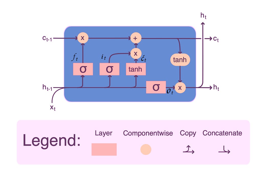
The LSTM consists of many memory blocks, as shown in the image is one whole block. Two states are carried over to the next block; cell state (stores and loads information) and hidden state (carries information from immediately previous events and overwrites). LSTMs learn using a process known as gates. These gates can learn which information in the sequence should be retained or dismissed. As a result, the LSTM contains three gates: input, forget, and output. More details on LSTM from here.

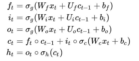
ft= Forget gate

it= Input gate

ot= Output gate

Ct= Cell state

ht= Hidden state

What is Bidirectional LSTM

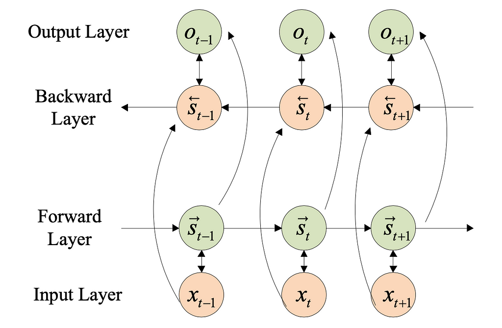
Bidirectional long-short term memory (BiLSTM) is the technique of allowing any neural network to store sequence information in both ways, either backward or forward. Our input runs in two ways in bidirectional, distinguishing a BiLSTM from a standard LSTM. We can have the input flow in both directions; to store past and future information at any time step. Nevertheless, normal LSTMs allow input flow in one direction (forward or backward).

What is NeuralProphet

NeuralProphet, a new open-source time series forecasting toolkit created using PyTorch, is based on neural networks. It is an enhanced version of Prophet (Automatic Forecasting Procedure), a forecasting library that allows you to utilize more advanced and sophisticated deep learning models for time series forecasting with the influence of AR-Net libraries (autoregressive neural network).

* Installing the latest version of the tool from GitHub using the following command and check the link below for NeuralProphet documentation.

#Use (!pip)if it did not install
pip install neuralprophet

#Live version(more features)if you are going to use the Jupyter
pip install neuralprophet[live]

GitHub – ourownstory/neural_prophet: NeuralProphet: A simple forecasting package

Let’s Get Started With the Stock Data

1. Data Preparation

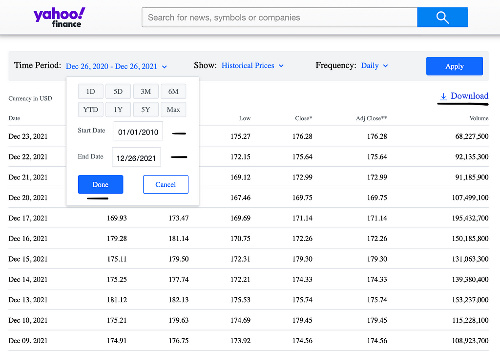
In this project, data are obtained from 2010–01–04 to 2021–11–02 for Apple Inc (AAPL) and exported directly from Yahoo finance. Stock price history will be for the past 11 years (including the Covid-19 period) since we use neural networks, and the more data, the better model training. As stated, the above-described models and tools will be applied to the “Date” of the dataset as univariate time series.

2. Data Preprocessing

• Import libraries

# Use Colab notebooks(recommended) or jupyterlab, etc.
import pandas as pd
import numpy as np
import seaborn as sns
import matplotlib.pyplot as plt
from matplotlib.pylab import rcParams
from datetime import datetime
import warnings
warnings.filterwarnings('ignore')
%matplotlib inline

• Read and explore data

# Reading the exported file as CSV. 
data = pd.read_csv("AAPL.csv")
print(data.head())

# Check duplicate, nan and so on. 
data.duplicated().sum().any()
data.isna().sum()

# Function to explore and validate
def explore(df):
   print(f"Dataset Shape: {df.shape}")
   summary = pd.DataFrame(df.dtypes,columns=['dtypes'])
   summary = summary.reset_index()
   summary['Name'] = summary['index']
   summary = summary[['Name','dtypes']]
   summary['Missing'] = df.isnull().sum().values
   summary['Uniques'] = df.nunique().values
   return summary

# function call
explore(data)

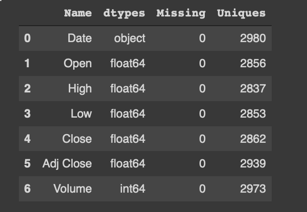
As you can see, after applying the explore function, the “Date” is an object type and need to be changed to the DateTime format as shown below:

# convert Date from object to datetime
data['Date'] = pd.to_datetime(data['Date'], infer_datetime_format=True)

# print info to check conversion 
data=data.set_index(['Date']) # set date as index or rest_index()
data.head()
print(data.info())

# Output:
Data columns (total 7 columns):
 #   Column     Non-Null Count  Dtype         
---  ------     --------------  -----         
 0   Date       2980 non-null   datetime64[ns]
 1   Open       2980 non-null   float64       
 2   High       2980 non-null   float64       
 3   Low        2980 non-null   float64       
 4   Close      2980 non-null   float64       
 5   Adj Close  2980 non-null   float64       
 6   Volume     2980 non-null   int64
 #   Column     Non-Null Count  Dtype         
---  ------     --------------  -----         

Model Implementation Phase

1. Stacked LSTM

After preprocessing the stock data, the “Adj Close” feature will be the target value. Due to this, “Adj Close” takes into account any factors (splits, dividends, and rights offerings) that may impact the stock price after the market closes.

Then, normalize the data using the MinMaxScaler function from sklearn before model fitting, it will boost and elevate the performance in Neural Networks.

• Let’s dive into the code:

It is now time to construct the Stacked LSTM (multiple layers) with an early stop to avoid overfitting if the validation loss has not reduced after a number of patience(no improvement after training).

Note: set a random seed (reproducible results) of TensorFlow if you want the same result each time to run your model without getting different results each run, or save the model or its weights for the best training to use later (more details on how to store and load models from here).

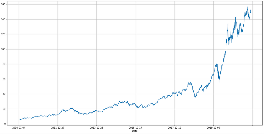
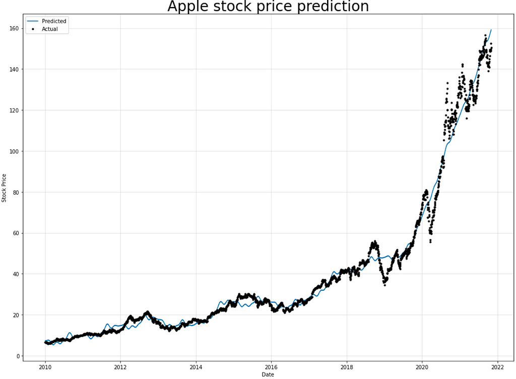
# The figure below of the real “Adj Close” feature of Apple stock from the dataset (y-axis is the stock price and x-axis is the date).

data.set_index('Date')['Adj Close'].plot(figsize=FIGURE_SIZE)

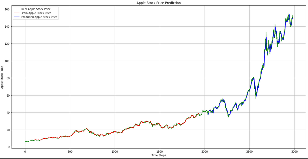
• Visualizing Stacked LSTM result

2. Bidirectional LSTM

Building the Bidirectional LSTM model with the same selected feature (adjusted closing price) from the Stacked LSTM dataset.

As seen below, one layer of BiLSTM was created utilizing the ReLU (Rectified Linear Unit) activation function. However, if the RMSProp (Root Mean Square Propagation) optimizer is applied, it will produce almost similar results as the Adam optimizer (used in BiLSTM building), and you may experiment with all of them.

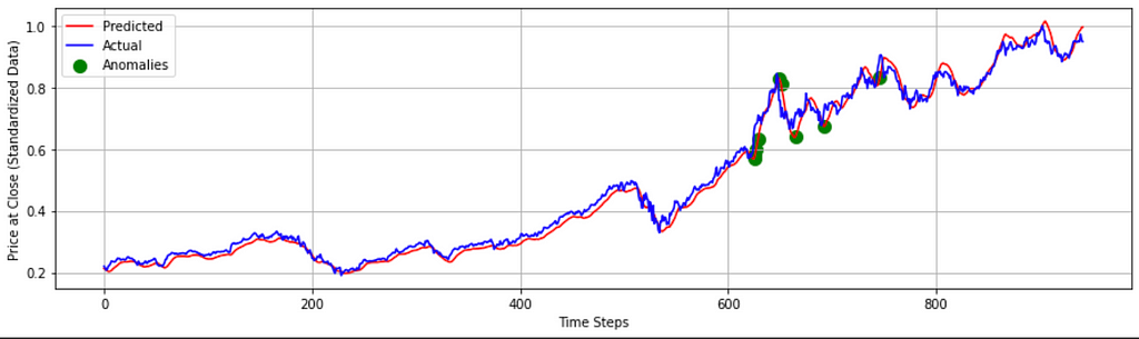
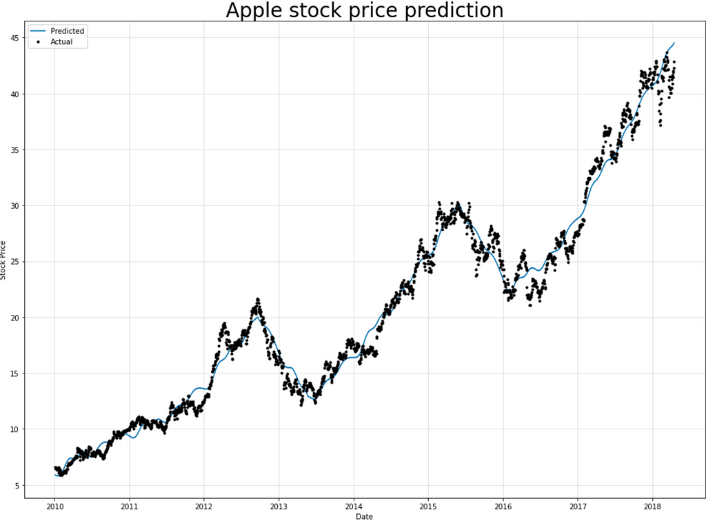
• Visualizing BiLSTM result

3. NeuralProphet

Finally, let’s start with NeuralProphet for modeling time-series based on neural networks.

• Install and import libraries as shown in this example:

The NeuralProphet model fit object assumes that the time series data has a date column named ds (date) and a time series value that you expect as y (predicted column name- Adj Close). Follow the below code:

Initialize the NeuralProphet model with default hyperparameters. And D frequency is used as the data based on daily adj-closing price.

Train the model with 1000 epochs (you can choose your epochs) which will take a few minutes for waiting, and NeuralProphet is fast on training to make predictions.

Plotting the forecast with more components, but what it will be shown as a result is model. plot(forecast).

• Visualizing gNeuralProphet result

In this code, splitting the dataset manually by NeuralProphet into training and testing to use 30% of train data as validation data.

• visualizing NeuralProphet result

Models Train & validation Loss

The learning curve is just a graph showing the progress of the experience of a particular indicator of learning during the training. To evaluate the model performance in prediction, look at the number of epochs in each model with its loss.

Note: Overfitting and underfitting are common, but excessive quantities must be controlled with strategies such as dropout to guarantee generalization. Therefore, the goal is to minimize the validation loss as much as possible until it reaches a good fitting with train loss. All implemented models in this post used an early stop to avoid overfitting.

• Stacked LSTM train & validation Loss:

RMSE (Root Mean Square Error) performance metrics:

Train Data: 20.75, Test Data: 80.098

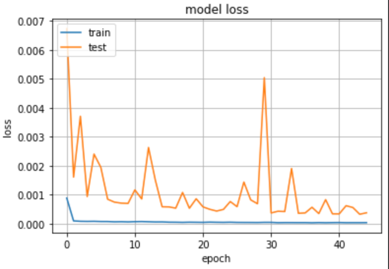
The fluctuation points at the end of the validation loss can be a point where learning can stop. Because experience after this point might show the complexities of overfitting.

• BiLSTM train & validation Loss:

RMSE performance metrics: Train Data: 20.288, Test Data: 87.739

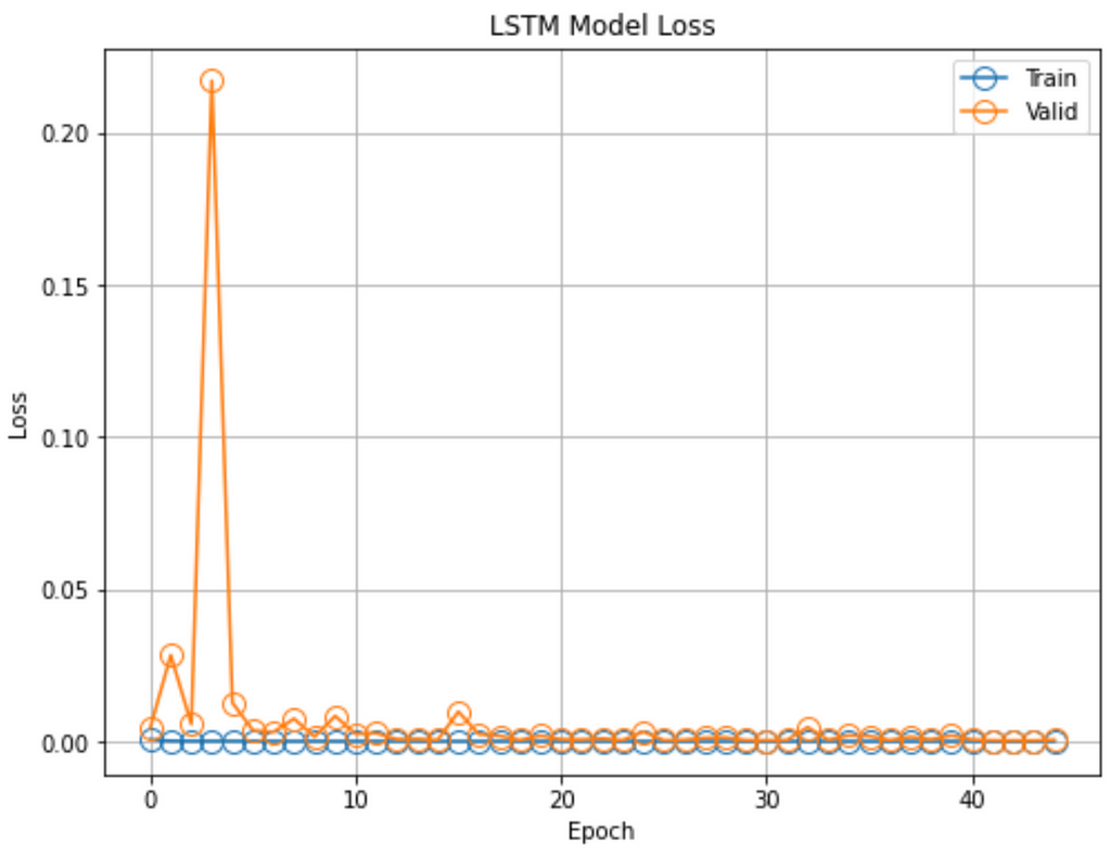
The graph shows how validation loss grew, then fell suddenly from large to small levels below 0.05 across three epochs. ReLU activation function is used to handle the vanishing/exploding gradient problem and might be caused the high pulsing in BiLSTM training.

• NeuralProphet train & validation Loss:

RMSE performance metrics: Train Data: 1.16, Test Data: 31.8

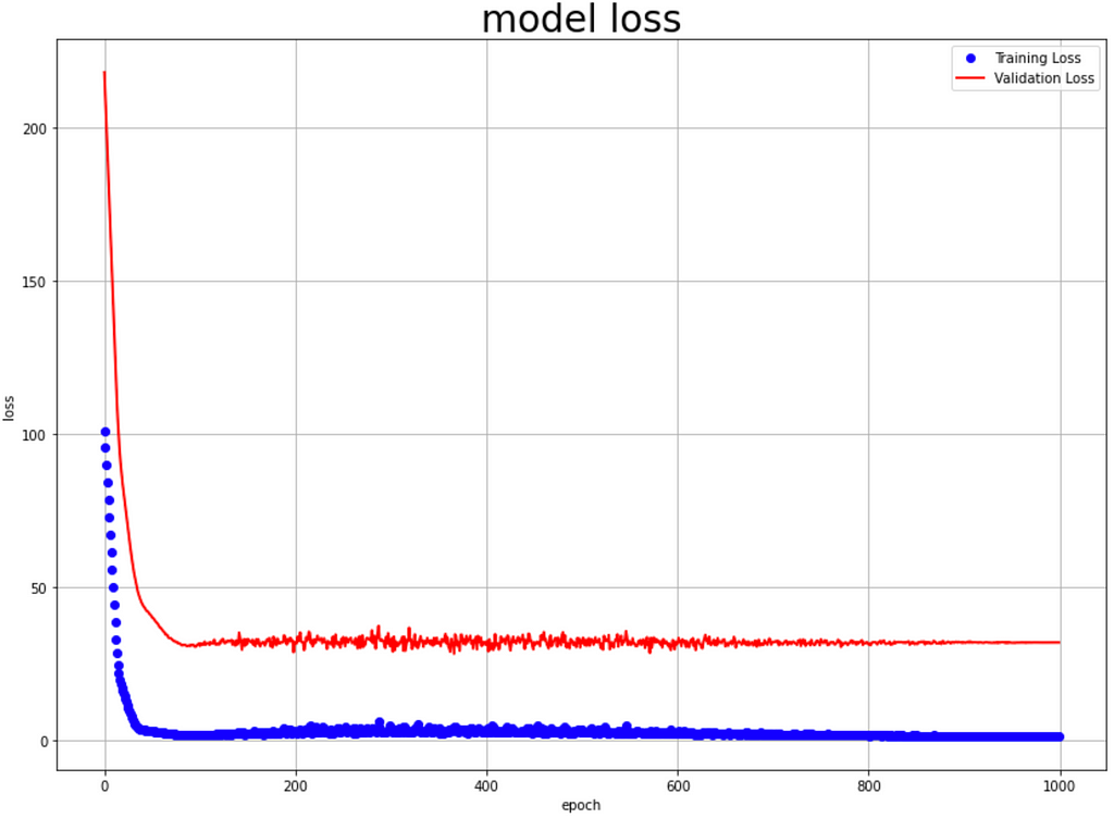
The train and validation loss are improving, but there is a gap between them, implying that they behave differently than datasets from various distributions.

Conclusion

As we can see, our models functioned admirably. It can accurately follow most unexpected jumps/drops from 2010 to 2021; however, you can enhance the performance by tinkering with the hyperparameters and adjusting even more. Several other actions can assist in fine-tuning the hyperparameters, such as changing the number of hidden layers, number of neurons, learning rate, activation function, and optimizer settings. But, these held for another discussion.

I hope you gained something by getting this far in understanding time-series forecasting using deep learning with the implementation of Stacked LSTM and BiLSTM models in Tensorflow, as well as exploring the NeuralProphet modeling library. Therefore, the models presented here can be used for a variety of additional time-series prediction scenarios where you can specify multivariate data as a 3D tensor.

If you have any comments or questions, please post them below. The whole Jupyter notebook for this project with EDA (Exploratory Data Analysis), visualization, transformation back to original form after training, performance metrics, future forecasting and more, is accessible on my GitHub repository.

All source code in this post and more can be found over at my GitHub at:

GitHub – A-safarji/Time-series-deep-learning: Developing Deep learning LSTM, BiLSTM models, and NeuralProphet for multi-step time-series forecasting of stock price.

Disclaimer: Attempts have been made to predict stock prices using time series analysis algorithms, but they are not available for betting in the real market. This is just a tutorial and implementation of deep learning models to forecast stock. Therefore, it is not intended to let others buy stock from this publishing.

😃 Thanks for your time. HAPPY LEARNING!

Reference

• Understanding Time Series
• What are Recurrent Neural Networks?

Cai C, Tao Y, Zhu T, Deng Z. Short-Term Load Forecasting Based on Deep Learning Bidirectional LSTM Neural Network. Applied Sciences. https://doi.org/10.3390/app11178129

• The Performance of LSTM and BiLSTM in Forecasting Time Series
• NeuralProphet documentation
• How to Develop LSTM Models for Time Series Forecasting – Machine Learning Mastery
• HOW TO PREVENT THE OVERFITTING | REGULARIZATION – PROGRAMMING REVIEW

---

Univariate Time Series With Stacked LSTM, BiLSTM, and NeuralProphet was originally published in Towards AI on Medium, where people are continuing the conversation by highlighting and responding to this story.

Join thousands of data leaders on the AI newsletter. It’s free, we don’t spam, and we never share your email address. Keep up to date with the latest work in AI. From research to projects and ideas. If you are building an AI startup, an AI-related product, or a service, we invite you to consider becoming a sponsor.

Published via Towards AI