


Explainable Defect Detection Using Convolutional Neural Networks: Case Study
Last Updated on January 17, 2022 by Editorial Team
Author(s): Olga Chernytska
Originally published on Towards AI the World’s Leading AI and Technology News and Media Company. If you are building an AI-related product or service, we invite you to consider becoming an AI sponsor. At Towards AI, we help scale AI and technology startups. Let us help you unleash your technology to the masses.
Deep Learning
Train object detection model without having any bounding boxes labels. This post shows the power of Explainable AI.
Despite being extremely accurate, neural networks are not that widely used in the domains, where prediction explainability is a requirement, such as medicine, banking, education, etc.
In this tutorial, I’ll show you how to overcome this explainability limitation for Convolutional Neural Networks. And it is — by exploring, inspecting, processing, and visualizing feature maps produced by deep neural network layers. We will go through the approach and discuss how to apply it to a real-world task — Defect Detection.
I’ve created a Github repository for this project, where you can find all data preparation, model, training, and evaluation scripts.
Contents
— Task
— Training Pipeline
— Inference Pipeline
— Evaluation
— Conclusion
Task
You are given a 400-image dataset, that contains images of good items (labeled as class ‘Good’) and items with a defect (labeled as class ‘Anomaly’). Dataset is imbalanced — with more samples of good images than defective ones. Item in the image may be literally of any type and complexity — bottle, cable, pill, tile, leather, zipper, etc. Below is an example of how the dataset may look like.
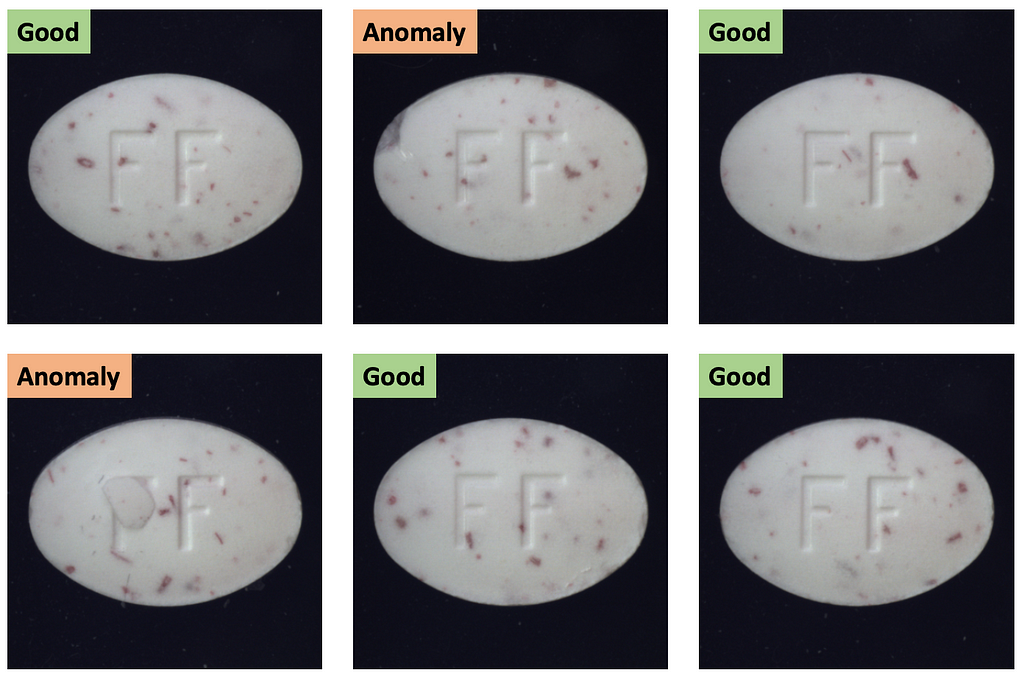
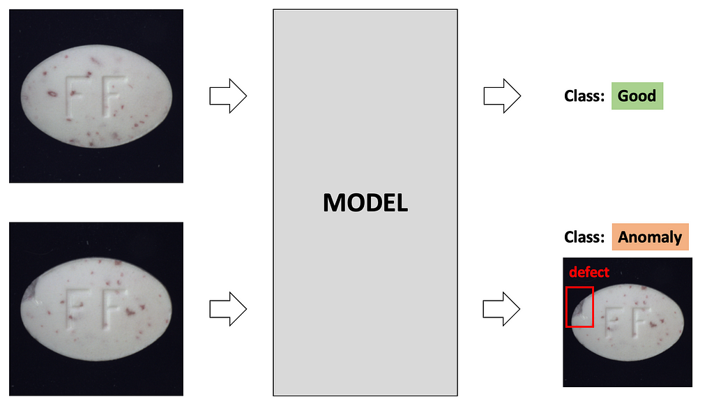
Your task is to build a model, that classifies images into ‘Good’ / ‘Anomaly’ classes and returns a bounding box for the defect if the image is classified as an ‘Anomaly’. Even though this task may look simple, like a typical object detection task, there is an issue — we do not have labels for bounding boxes.
Fortunately, this task is solvable.
Training Pipeline
Disclosure: I am not sharing my real commercial project, but showing how to explain the classification model predictions in general, so this may be used in many domains and tasks — not only manufacturing but medicine as well. I should also say that do not expect high accuracy here, because it’s my quick pet project. But you are free to use my results as a starting point for your project, invest more time and achieve the accuracy you need : )
Data Preparation
For all my experiments I’ve used MVTEC Anomaly Detection Dataset (pay attention, it is distributed under Creative Commons Attribution-NonCommercial-ShareAlike 4.0 International License, which means that it cannot be used for commercial purposes).
The dataset includes 15 subsets of different item types, such as Bottle, Cable, Pill, Leather, Tile, etc; each subset has 300–400 images total — each labeled as ‘Good’/’Anomaly’.
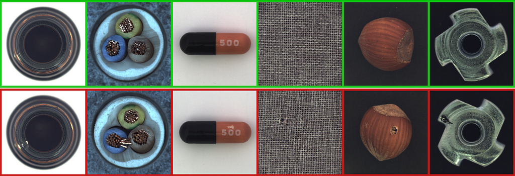
upper row — good images, lower row — images with the defective items. Image Source
As a data preprocessing step, resize images to 224×224 pixels to speed up training. Images in most subsets are of size 1024×1024, but as defects are also of the large size, we may resize the image to a lower resolution without sacrificing model accuracy.
Consider using Data Augmentations. In general, appropriate data augmentations are ALWAYS beneficial for your model (BTW, check my post on data augmentation to learn more).
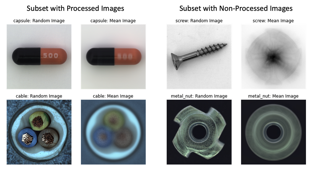
But let’s assume that when deployed to production our model will “see” the data of exactly the same format as in the dataset we have now. So, if images are centered, scaled, and rotated (as in Capsule and Cable subsets), we may not use any data augmentations at all, because test images are expected to be also centered, scaled, and rotated. However, if mages are not rotated (but only centered and scaled), as in Screw and Metal Nut subsets, adding Rotation as a preprocessing step to the training pipeline would help the model learn better.
Split the data into train/test parts. Ideally, we would like to have train, validation, and test parts — to train a model, tune hyperparameters and evaluate model accuracy, respectively. But we have only 300–400 images, so let’s put 80% of images into the train set and 20% — into the test set. For small datasets, we may perform 5-Fold cross-validation to make sure that evaluation results are robust.
When dealing with an imbalanced dataset, train/test split should be performed in a stratified manner, so train and test parts will contain the same share of both classes — ‘Good’/’Anomaly’. Additionally, if you have information on the defect types (such as scratch, crack, etc), it’s better to do a stratified split based also on defect types, so train and test parts will contain the same share of items with scratches/cracks.
Model
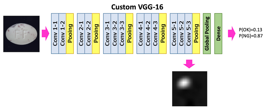
Let’s take VGG16 pre-trained on ImageNet, and change its classification head — replace Flattening and Dense layers with Global Average Pooling and a single Dense layer. I’ll explain in section “Inference Pipeline” why we need these particular layers.
(This approach I’ve found in the paper Learning Deep Features for Discriminative Localization. In this post, I’ll go through all the important steps described in the paper.)
We train the model as a typical 2-class classification model. The model outputs a 2-dimensional vector that contains probabilities for classes ‘Good’ and ‘Anomaly’ (with 1-dimensional output, the approach should also work, feel free to try).
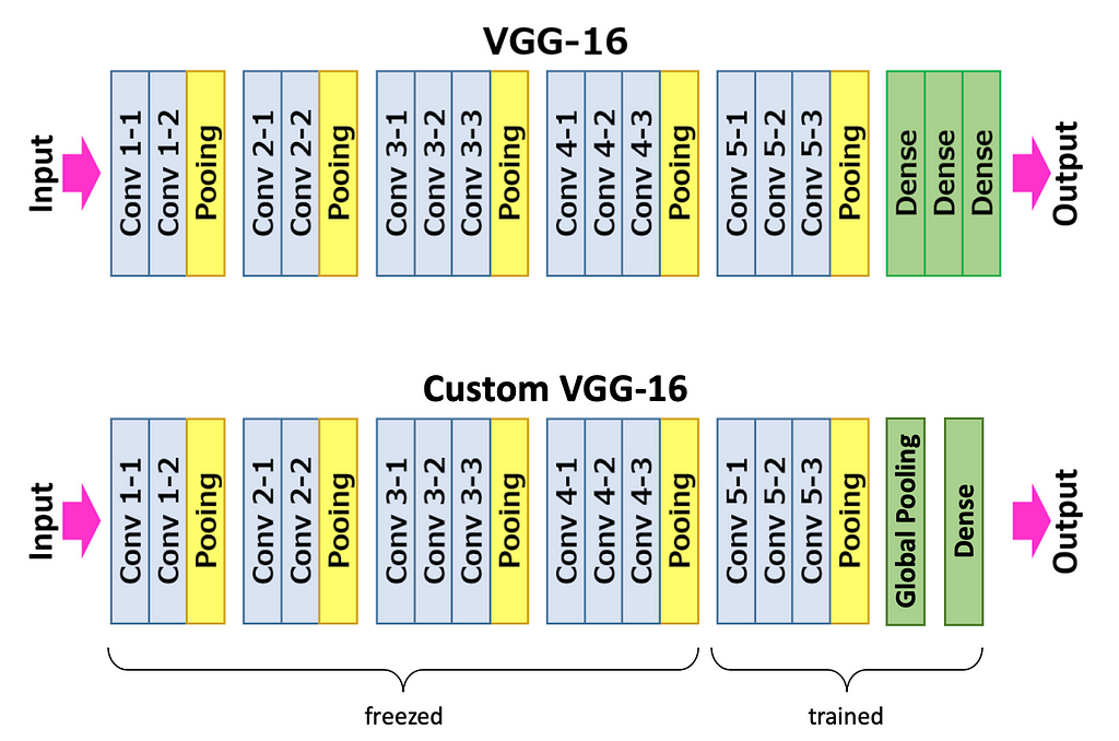
During training, the first 10 convolutional layers are frozen, we train only the classification head and the last 3 convolutional layers. That’s is because our dataset is too small to finetune the whole model. Loss is Cross-Entropy; optimizer is Adam with a learning rate of 0.0001.
I’ve experimented with different subsets of the MVTEC Anomaly Detection Dataset. I’ve trained the model with batch_size=10 for at most 10 epochs and early stopping when train set accuracy reaches 98%. To deal with the imbalanced dataset, we may apply loss weighting: use higher weight for ‘Anomaly’ class images and lower — for ‘Good’.
Inference Pipeline
During inference, we want not only to classify an image into ‘Good’ / ‘Anomaly’ classes but also to get a bounding box for the defect if the image is classified as an ‘Anomaly’.
For this reason, we make the model in inference mode to output class probabilities as well as the heatmap, which later will be processed into the bounding box. Heatmap is created from the feature maps from deep layers.
Step 1. Take all feature maps from Conv5–3 layer, after ReLU activation. For a single input, there will be 512 feature maps of size 14×14 (input image of size 224×224 was downsampled each time twice by 4 Pooling layers).
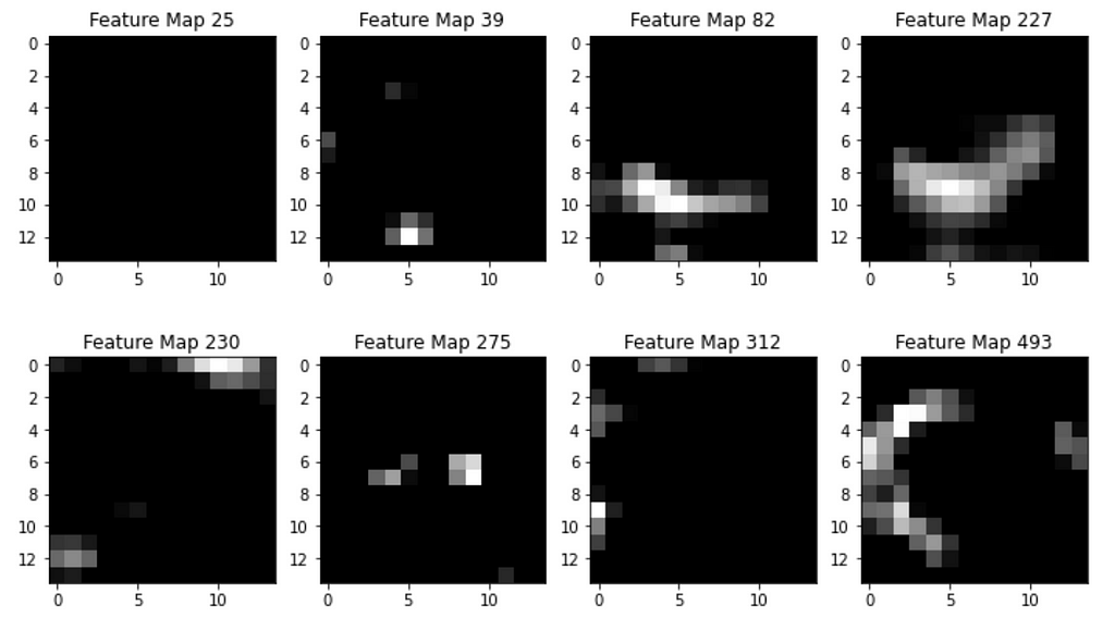
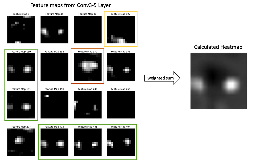
There are 512 feature maps total, each of size 14×14; visualized only some of them. Image by Author
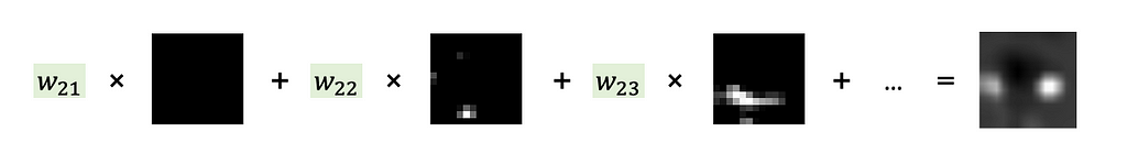
Step 2. Sum up all 512 feature maps from the Conv5–3 layer each multiplied by the weight in the Dense layer that affected the calculation of the ‘Anomaly’ class score. Carefully look at Images 7 and 8 to understand this step.
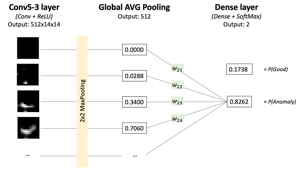
Why so? Now you’ll see why the classification head should have a Global Average Pooling Layer and a Dense Layer. Such architecture makes it possible to follow, what feature maps (and how much) affected the final prediction and made it to be an ‘Anomaly’ class.
Each feature map (output of layer Conv5–3; see Image 6) highlights some regions in the input image. The Global Average Pooling layer represents each feature map as a single number (we may think about it as 1-D embedding). The dense layer calculates scores (and probabilities) for classes ‘Good’ and ‘Anomaly’ by multiplying each embedding by the corresponding weight. This flow is shown in Image 7.
So Dense layer weights represent how much each feature map affects the scores for ‘Good’ and ‘Anomaly’ classes (we are interested in the ‘Anomaly’ class score only). And summing up feature maps from layer Conv5–3 each multiplied by corresponding weight from the Dense layer — makes a lot of sense.
Interestingly, using Global Average Pooling but not Global Max Pooling is crucial to make the model find the whole object. Here is what the original paper Learning Deep Features for Discriminative Localization says:
“We believe that Global Average Pooling loss encourages the network to identify the extent of the object as compared to Global Max Pooling which encourages it to identify just one discriminative part. This is because, when doing the average of a map, the value can be maximized by finding all discriminative parts of an object as all low activations reduce the output of the particular map. On the other hand, for Global Max Pooling, low scores for all image regions except the most discriminative one do not impact the score as you just perform a max.”
Step 3. The next step is to upsample the heatmap to match the input image size — 224×224. Bilinear upsampling is okay, like any other upsampling method.
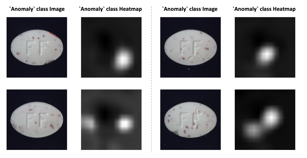
Coming back to the model output. The model returns probabilities for classes ‘Good’ and ‘Anomaly’ and a heatmap that shows what pixels were important when calculating the ‘Anomaly’ score. Models return the heatmap always, no matter it classified the image as ‘Good’ or ‘Anomaly’; when class is ‘Good’ — we just ignore the heatmap.
The heatmaps look quite well (see Image 11), and explain what region made the model decide that the image belongs to the ‘Anomaly’ class. We may stop here, or (as I promised) process the heatmap into a bounding box.
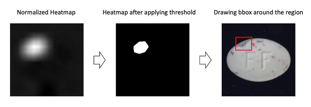
From heatmaps to bounding boxes. You may come up with several approaches here. I’ll show you the simplest one. In most cases, it works pretty well.
1. First, normalize the heatmap, so all the values are in the range [0,1].
2. Select a threshold. Apply it to the heatmap, so all values larger than the threshold are transformed into 1s and smaller — into 0s. The larger the threshold — the smaller the bounding box will be. I like how the results look when the threshold is in the range [0.7, 0.9].
3. We assume, that region of 1s — is a single dense region. Then plot a bounding box around the region, by finding argmin and argmax in heights and width dimensions.
However, pay attention that this approach can only return a single bounding box (by definition), so it would fail if the image has multiple defective regions.
Evaluation
Let’s evaluate the approach on 5 subsets from the MVTEC Anomaly Detection Dataset — Hazelnut, Leather, Cable, Toothbrush, and Pill.
For each subset, I’ve trained a separate model; 20% of images were selected as a test set — randomly and in a stratified manner. No data augmentations were used. I applied class weighing in loss function — 1 for ‘Good’ class and 3 for ‘Anomaly’, because in most subsets there are 3 times more good images than anomalous ones. The model was trained for at most 10 epochs with early stopping if train set accuracy reaches 98%. Here is my notebook with the training script.
Below are the evaluation results. Train set size for subsets is 80–400 images. Balanced Accuracy is between 81.7% and 95.5%. Some subsets, such as Hazelnut and Leather, are easier for models to learn, while Pill is a relatively hard subset.
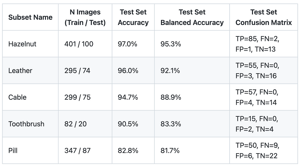
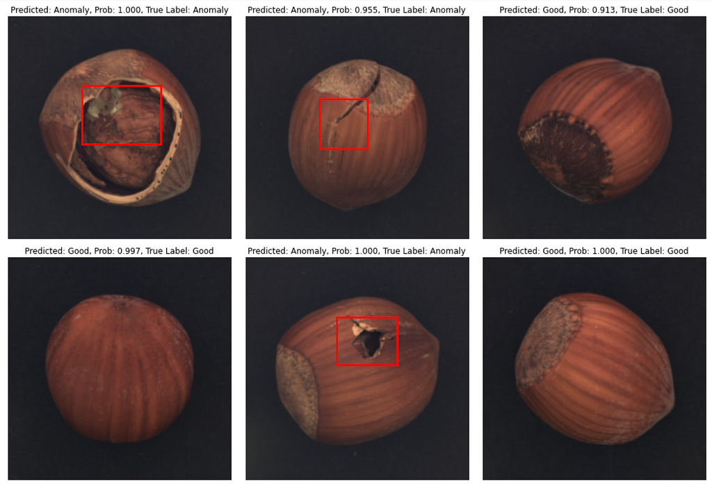
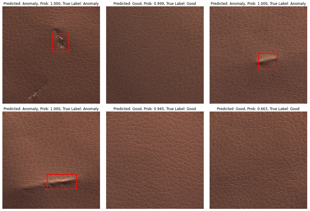
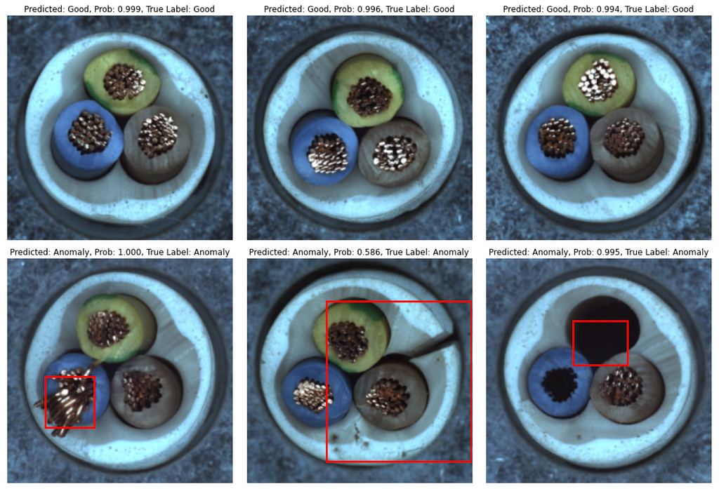
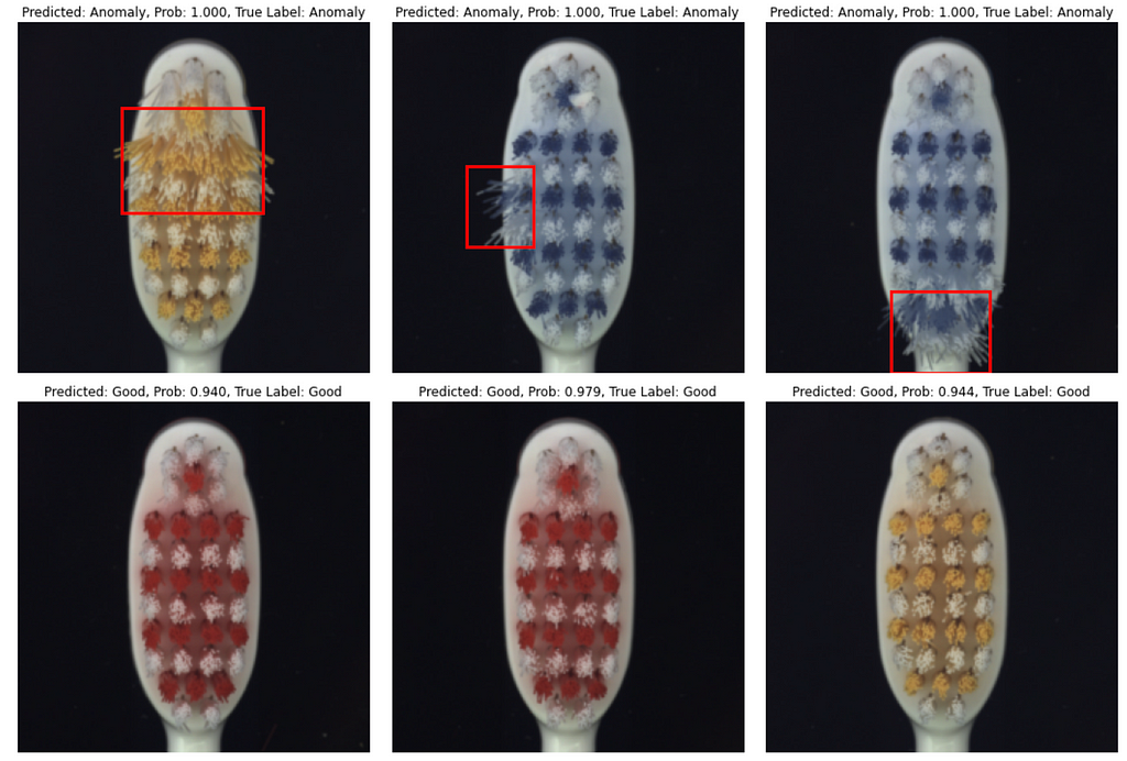
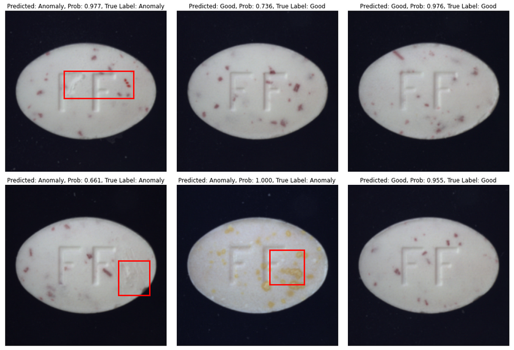
That’s it with numbers, and now let’s see how predictions look like. In most cases model produces correct class prediction and precise bounding box if the class is an ‘Anomaly’. However, there are some errors: they are either incorrect class prediction or wrong bounding box location when class is correctly predicted as an ‘Anomaly’.
Conclusion
In this post, I wanted to show you that neural networks are not black-box algorithms as some may think, but are quite explainable when you know where to look 🙂 And the approach described here is one of the many ways of how to explain your model predictions.
Of course, the model is not that accurate, mostly because it is my quick pet project. But if you would work on a similar task, feel free to take my results as a starting point, invest more time and get the accuracy you need.
I am open-sourcing the code for this project to this Github repository. Feel free to use my results as a starting point for your project 🙂
What’s next?
If you’d like to improve the accuracy of this Anomaly Detection model, adding data augmentation — is the place to start. I recommend you to read my post — Complete Guide to Data Augmentation for Computer Vision. There you’ll find how to use Data Augmentations to benefit your model, and not to do harm 🙂
In case you are interested in case studies, check my tutorial — Gentle introduction to 2D Hand Pose Estimation: Approach Explained.
And subscribe to my Twitter or Telegram not to miss my new posts 🙂
References
[1] Zhou, Bolei, Aditya Khosla, Agata Lapedriza, Aude Oliva, and Antonio Torralba: Learning deep features for discriminative localization; in: Proceedings of the IEEE conference on computer vision and pattern recognition, 2016. pdf
[2] Paul Bergmann, Kilian Batzner, Michael Fauser, David Sattlegger, Carsten Steger: The MVTec Anomaly Detection Dataset: A Comprehensive Real-World Dataset for Unsupervised Anomaly Detection; in: International Journal of Computer Vision, January 2021. pdf
[3] Paul Bergmann, Michael Fauser, David Sattlegger, Carsten Steger: MVTec AD — A Comprehensive Real-World Dataset for Unsupervised Anomaly Detection; in: IEEE Conference on Computer Vision and Pattern Recognition (CVPR), June 2019. pdf
Explainable Defect Detection Using Convolutional Neural Networks: Case Study was originally published in Towards AI on Medium, where people are continuing the conversation by highlighting and responding to this story.
Join thousands of data leaders on the AI newsletter. It’s free, we don’t spam, and we never share your email address. Keep up to date with the latest work in AI. From research to projects and ideas. If you are building an AI startup, an AI-related product, or a service, we invite you to consider becoming a sponsor.
Published via Towards AI
Towards AI Academy
We Build Enterprise-Grade AI. We'll Teach You to Master It Too.
15 engineers. 100,000+ students. Towards AI Academy teaches what actually survives production.
Start free — no commitment:
→ 6-Day Agentic AI Engineering Email Guide — one practical lesson per day
→ Agents Architecture Cheatsheet — 3 years of architecture decisions in 6 pages
Our courses:
→ AI Engineering Certification — 90+ lessons from project selection to deployed product. The most comprehensive practical LLM course out there.
→ Agent Engineering Course — Hands on with production agent architectures, memory, routing, and eval frameworks — built from real enterprise engagements.
→ AI for Work — Understand, evaluate, and apply AI for complex work tasks.
Note: Article content contains the views of the contributing authors and not Towards AI.
Related posts
Recent Posts


")

