Random_Forest_Medium_Article

Author(s): Jatindeep Singh

Originally published on Towards AI the World’s Leading AI and Technology News and Media Company. If you are building an AI-related product or service, we invite you to consider becoming an AI sponsor. At Towards AI, we help scale AI and technology startups. Let us help you unleash your technology to the masses.

Credit Default Modelling Using Decision Trees

Detecting Credit Worthiness using Tree-based techniques

Machine Learning Algorithms have historically been used in the Credit and Fraud Space. With the increase in computational power, the Industry has made a move from Tree-based Logit models to more advanced Machine Learning Techniques involving Bagging and Boosting. industry. The article is designed to provide the readers with a Mathematical View of Decision Trees, Bagging, and Random Forest Algorithms. In the final section, the writer discusses how to use these techniques for Credit Default and Fraud Prevention using Data from LendingClub.

Decision Trees

1. Introduction

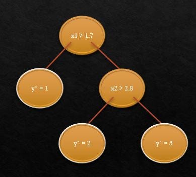
The basic intuition behind decision trees is to map out all possible decision paths in the form of a binary tree. Showcasing the same with the example of identifying flower type(y) using the ratio of sepal length to width(x1) and the ratio of petal length to width(x2)

The initial split at x1>1.7 helps in identifying flower type y=1

The next node split at x2>2.8 helps identify y=2 and y=3

Mathematically, a Decision Tree maps inputs x ∈ R^d to output y using binary decision rules:

Each node in the tree has a splitting Rule

• Splitting based on top-down Greedy Algorithm
• Each Leaf Node is associated with an output value

Each splitting rule is of the form

• h(x) = 1{xj > t}

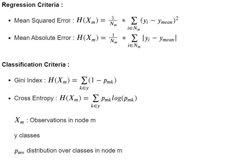
2. Splitting Criteria

3. Geometrical View

Motivation :

• Partition the space so that data in a region have the same prediction
• Each partition represents a vertical or horizontal line in the 2-D plane

4. Challenges

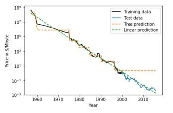
• Decision Trees cannot Extrapolate

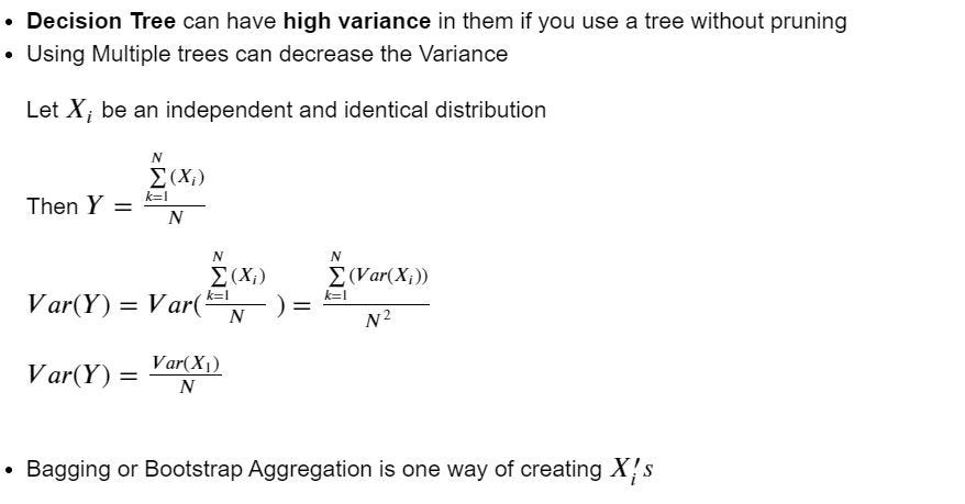
• High Variance or Instability to change in data: By minor change in data we see the variation in the Structure of the Decision Tree
• The reason for the High Variance in decision trees lies in the fact that they are based on a Greedy Algorithm. It focuses on optimizing for the node split at hand, rather than taking into account how that split impacts the entire tree. A greedy approach makes Decision Trees run faster but makes them prone to overfitting.

In the next sections, we will discuss how to overcome these challenges

Bootstrap Aggregator

1. Motivation

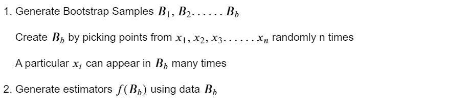
2. Algorithm

Random Forest

1. Motivation

2. Algorithm

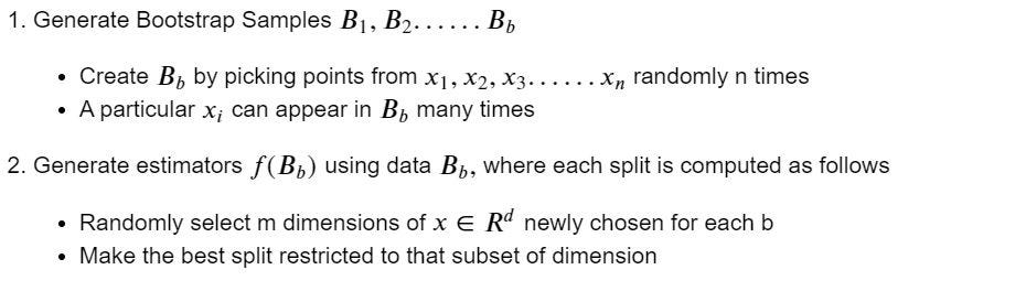
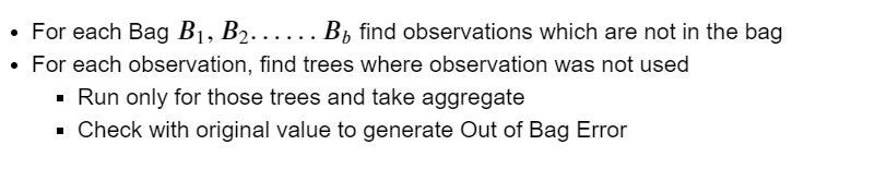
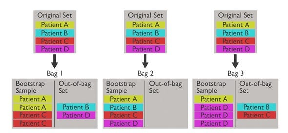
Another advantage of Random Forest is that it does not require a holdout dataset and hence can effectively work on smaller datasets. Instead of Test Errors, we can calculate Out of Bag (OOB) Errors. The framework for this is shown below :

3. Out of Bag Error

Jupyter Lab

Here we explore data from LendingClub.com

Given many different factors including the FICO score of the borrower, the interest rate, and even the purpose of the loan, we attempt to make predictions on whether a particular loan would be paid back in full.

Why Decision Trees / Random Forests?

Decision trees are a great ‘rough and ready’ ML technique that can be applied to many different scenarios. They are intuitive, and fast, and they can deal with both numerical and categorical data. The biggest drawback of Decision Trees is their tendency to overfit the given data, resulting in errors in either variance or bias. Random forests combat this problem by employing many different Decision Trees on random samples of the data, and so are usually a more sensible choice when choosing an ML model.

Imports

import pandas as pd
import numpy as np
import seaborn as sns
import matplotlib.pyplot as plt
%matplotlib inline

Exploratory Analysis

loans = pd.read_csv('loan_data.csv')

loans.head()

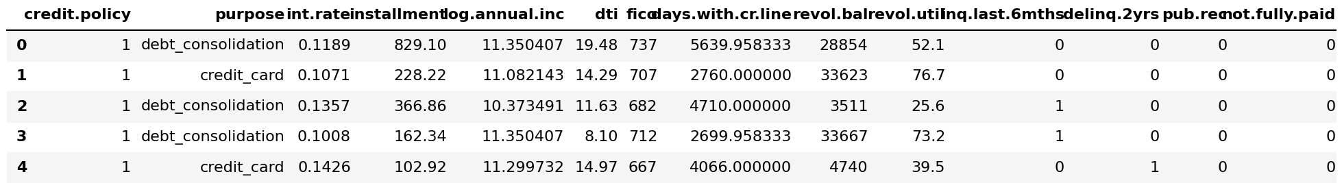
The ‘not.fully.paid’ column is the one we are interested in predicting.

loans.info()

<class 'pandas.core.frame.DataFrame'>
RangeIndex: 9578 entries, 0 to 9577
Data columns (total 14 columns):
 #   Column             Non-Null Count  Dtype  
---  ------             --------------  -----  
 0   credit.policy      9578 non-null   int64  
 1   purpose            9578 non-null   object 
 2   int.rate           9578 non-null   float64
 3   installment        9578 non-null   float64
 4   log.annual.inc     9578 non-null   float64
 5   dti                9578 non-null   float64
 6   fico               9578 non-null   int64  
 7   days.with.cr.line  9578 non-null   float64
 8   revol.bal          9578 non-null   int64  
 9   revol.util         9578 non-null   float64
 10  inq.last.6mths     9578 non-null   int64  
 11  delinq.2yrs        9578 non-null   int64  
 12  pub.rec            9578 non-null   int64  
 13  not.fully.paid     9578 non-null   int64  
dtypes: float64(6), int64(7), object(1)
memory usage: 1.0+ MB

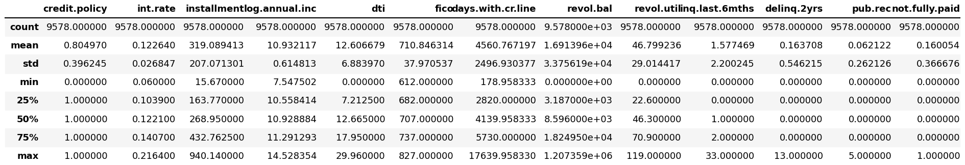
loans.describe()

Some columns Information

• credit.policy: 1 if the customer meets the credit underwriting criteria of LendingClub.com, and 0 otherwise.
• purpose: The purpose of the loan (takes values “credit_card”, “debt_consolidation”, “educational”, “major_purchase”, “small_business”, and “all_other”).
• int.rate: The interest rate of the loan, as a proportion (a rate of 11% would be stored as 0.11). Borrowers judged by LendingClub.com to be riskier are assigned higher interest rates.
• installment: The monthly installments owed by the borrower if the loan is funded.
• log.annual.inc: The natural log of the self-reported annual income of the borrower.
• dti: The debt-to-income ratio of the borrower (amount of debt divided by annual income).
• fico: The FICO credit score of the borrower.
• days.with.cr.line: The number of days the borrower has had a credit line.
• revol.bal: The borrower’s revolving balance (amount unpaid at the end of the credit card billing cycle).
• revol.util: The borrower’s revolving line utilization rate (the amount of the credit line used relative to total credit available).
• inq.last.6mths: The borrower’s number of inquiries by creditors in the last 6 months.
• delinq.2yrs: The number of times the borrower had been 30+ days past due on a payment in the past 2 years.
• pub.rec: The borrower’s number of derogatory public records (bankruptcy filings, tax liens, or judgments).

Data visualization

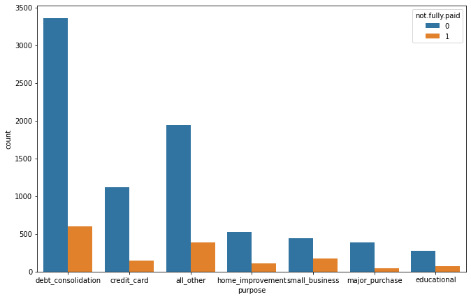
plt.figure(figsize=(11,7))
sns.countplot(loans['purpose'], hue = loans['not.fully.paid'])

We split our target function with respect to the purpose for which a loan was taken. 

new_df = loans.groupby('purpose')['not.fully.paid'].value_counts(normalize=True)
new_df = new_df.mul(100).rename('Percent').reset_index()

new_df1 = new_df[new_df["not.fully.paid"]==1]

new_df1=new_df1.sort_values("Percent")

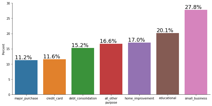
g=sns.catplot(x="purpose", y='Percent', kind='bar', data=new_df1, aspect=2)
g.ax.set_ylim(0,30)


for p in g.ax.patches:
    txt = str(p.get_height().round(1)) + '%'
    txt_x = p.get_x()
    txt_y = p.get_height()
    g.ax.text(txt_x,txt_y,txt,fontsize=18,verticalalignment='bottom',multialignment='right')

We would like to understand the risk as a percentage hence we look at proportion of unpaid loans in each purpose type

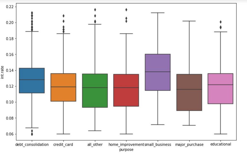
sns.boxplot(data =loans, x ='purpose', y= loans['int.rate']).legend().set_visible(False)

Given the knowledge of risk basis purpose, we would like to understand if the APR offered to a customer take into account purpose. 

df=loans
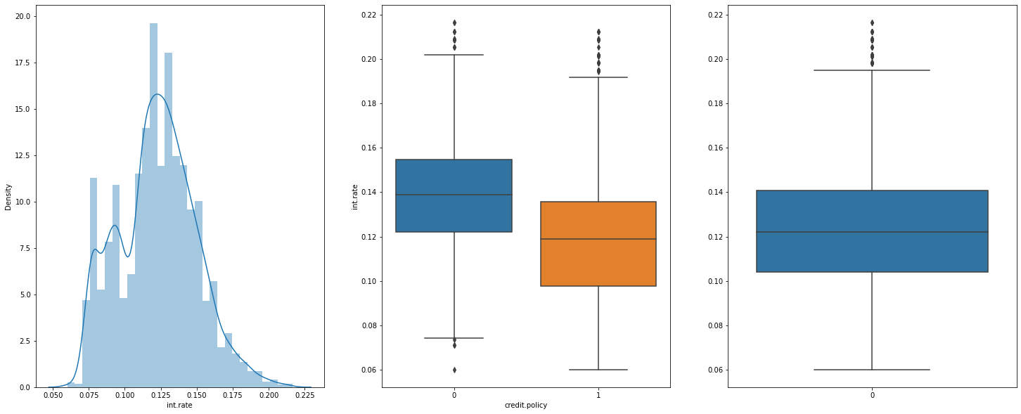
f,(ax1,ax2,ax3)= plt.subplots(1,3,figsize=(25,10))
sns.distplot(df['int.rate'], bins= 30,ax=ax1)
sns.boxplot(data =df, x ='credit.policy', y= df['int.rate'],ax=ax2).legend().set_visible(False)
sns.boxplot(data = df['int.rate'], ax=ax3)
print("Interest Rate Distribution, Credit Policy range based on the Credit policy , General Interest rate")

Interest Rate Distribution, Credit Policy range based on the Credit policy , General Interest rate

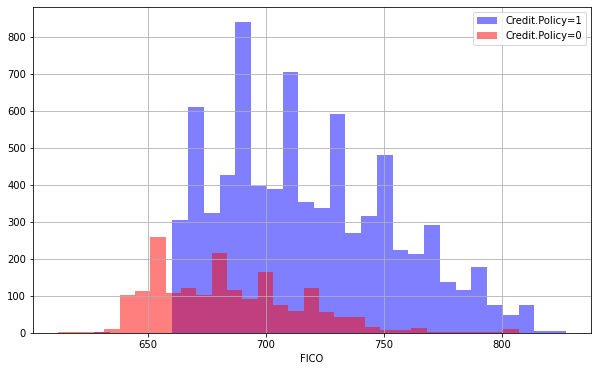
plt.figure(figsize=(10,6))
loans[loans['credit.policy']==1]['fico'].hist(alpha=0.5,color='blue',
                                              bins=30,label='Credit.Policy=1')
loans[loans['credit.policy']==0]['fico'].hist(alpha=0.5,color='red',
                                              bins=30,label='Credit.Policy=0')
plt.legend()
plt.xlabel('FICO')

Text(0.5, 0, 'FICO')

To understand if Credit Policy Underwriting from Lending Club have FICO based cut-off for applying customers, we look at the following histogram. 

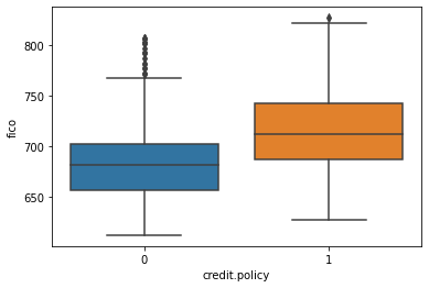
sns.boxplot(data =loans, x ='credit.policy', y= loans['fico']).legend().set_visible(False)

Credit Policy promotes individuals with Higher FICO 

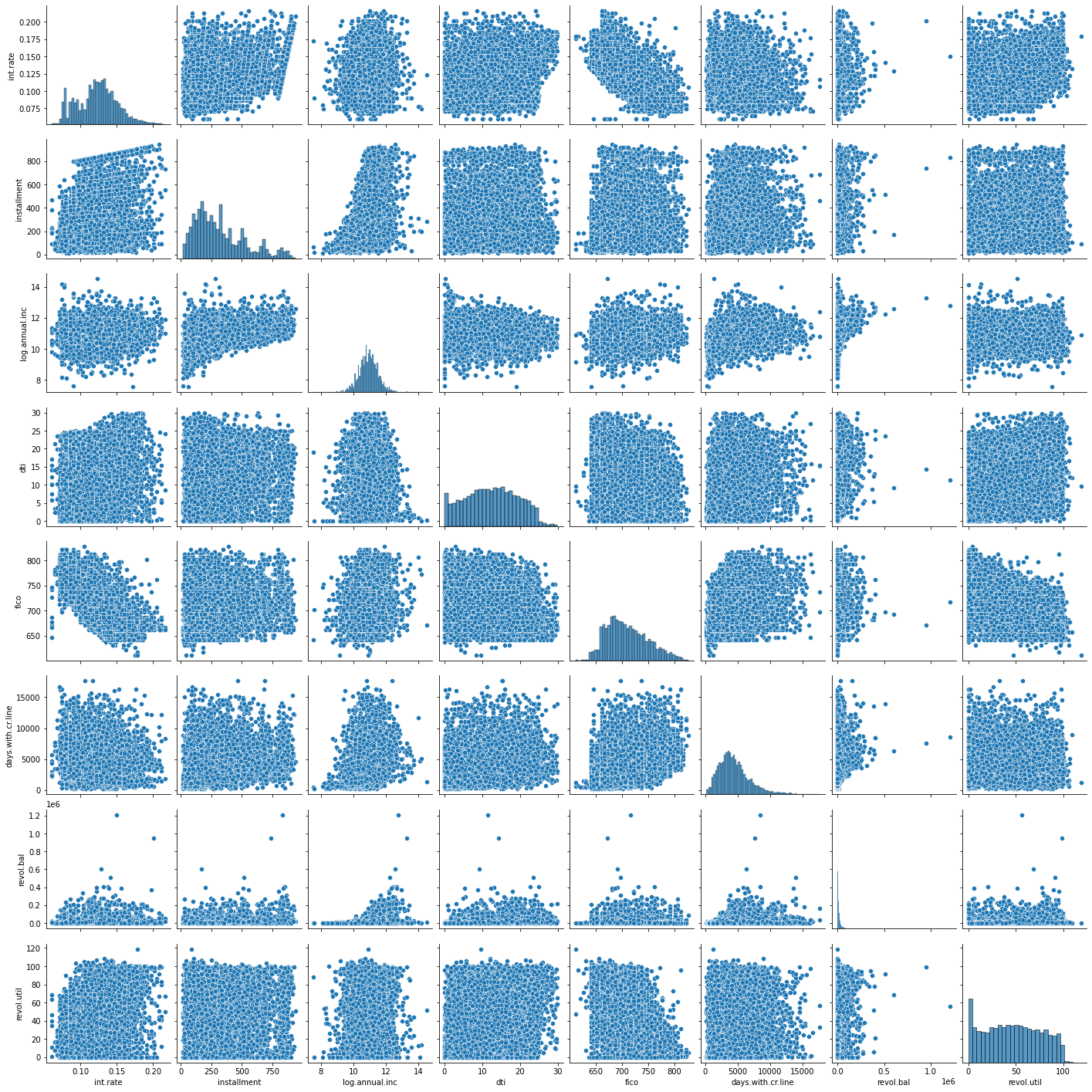
Let’s plot a seaborn pairplot between the numerical data:

sns.pairplot(loans.drop(['credit.policy', 'purpose',
       'inq.last.6mths', 'delinq.2yrs', 'pub.rec', 'not.fully.paid'], axis=1))

<seaborn.axisgrid.PairGrid at 0x1d9e00432c8>

Cleaning

Let’s transform the ‘purpose’ column to dummy variables so that we can include them in our analysis:

final_data = pd.get_dummies(loans,columns = ['purpose'], drop_first=True)

final_data.head()

from sklearn.model_selection import train_test_split

X= final_data.drop('not.fully.paid', axis=1)
y= final_data['not.fully.paid']
X_train, X_test, y_train, y_test = train_test_split(X,y,test_size = 0.3, random_state = 101)

Decision Tree:

from sklearn.tree import DecisionTreeClassifier

dtree = DecisionTreeClassifier(class_weight=None, criterion='gini', max_depth=None,
            max_features=None, max_leaf_nodes=None,
            min_impurity_decrease=0.0, min_impurity_split=None,
            min_samples_leaf=1, min_samples_split=2,
            min_weight_fraction_leaf=0.0,  random_state=None,
            splitter='best')

dtree.fit(X_train, y_train)

DecisionTreeClassifier()

pred = dtree.predict(X_test)

Evaluation

np.array((pred==y_test)).sum()

2104

from sklearn.metrics import classification_report, confusion_matrix

print(classification_report(y_test,pred))

precision    recall  f1-score   support

           0       0.86      0.82      0.84      2431
           1       0.19      0.23      0.21       443

    accuracy                           0.73      2874
   macro avg       0.52      0.53      0.53      2874
weighted avg       0.75      0.73      0.74      2874

print(confusion_matrix(y_test,pred))

[[2000  431]
 [ 339  104]]

Random Forest:

from sklearn.ensemble import RandomForestClassifier

dfor = RandomForestClassifier()

dfor.fit(X_train, y_train)

RandomForestClassifier()

pred2 = dfor.predict(X_test)

Evaluation

(y_test == pred2).sum()

2427

We can see that this has made a better prediction than a single tree

print(classification_report(y_test,pred2))

precision    recall  f1-score   support

           0       0.85      0.99      0.92      2431
           1       0.42      0.02      0.05       443

    accuracy                           0.84      2874
   macro avg       0.64      0.51      0.48      2874
weighted avg       0.78      0.84      0.78      2874

print(confusion_matrix(y_test,pred2))

[[2416   15]
 [ 432   11]]

Hyper Parameter Tuning ~ Random Forest

• n_estimators : Number of Trees in Random Forest
• max_features : Max Number of Features to be considered at each split
• max_depth : Max Depth of each estimator
• min_sample_split : Minimum Samples required for Valid Split
• min_samples_leaf : Minimum samples required at each leaf node

from sklearn.model_selection import RandomizedSearchCV
# Number of trees in random forest
n_estimators = [int(x) for x in np.linspace(start = 200, stop = 2000, num = 10)]
# Number of features to consider at every split
max_features = ['auto', 'sqrt']
# Maximum number of levels in tree
max_depth = [int(x) for x in np.linspace(10, 110, num = 11)]
max_depth.append(None)
# Minimum number of samples required to split a node
min_samples_split = [2, 5, 10]
# Minimum number of samples required at each leaf node
min_samples_leaf = [1, 2, 4]
# Create the random grid
random_grid = {'n_estimators': n_estimators,
               'max_features': max_features,
               'max_depth': max_depth,
               'min_samples_split': min_samples_split,
               'min_samples_leaf': min_samples_leaf,
               }
print(random_grid)

{'n_estimators': [200, 400, 600, 800, 1000, 1200, 1400, 1600, 1800, 2000], 'max_features': ['auto', 'sqrt'], 'max_depth': [10, 20, 30, 40, 50, 60, 70, 80, 90, 100, 110, None], 'min_samples_split': [2, 5, 10], 'min_samples_leaf': [1, 2, 4]}

K-Fold Cross-Validation

The technique of cross-validation (CV) is best explained by example using the most common method, K-Fold CV. When we approach a machine learning problem, we make sure to split our data into a training and a testing set. In K-Fold CV, we further split our training set into K number of subsets, called folds. We then iteratively fit the model K times, each time training the data on K-1 of the folds and evaluating on the Kth fold (called the validation data).

# Use the random grid to search for best hyperparameters
# First create the base model to tune
rf = RandomForestClassifier()
# Random search of parameters, using 3 fold cross validation, 
# search across 100 different combinations, and use all available cores
rf_random = RandomizedSearchCV(estimator = rf, param_distributions = random_grid, n_iter = 100, cv = 3, verbose=2, random_state=42, n_jobs = -1)
# Fit the random search model
rf_random.fit(X_train, y_train)

Fitting 3 folds for each of 100 candidates, totalling 300 fits





RandomizedSearchCV(cv=3, estimator=RandomForestClassifier(), n_iter=100, n_jobs=-1,
param_distributions={'max_depth': [10, 20, 30, 40, 50, 60,
                           70, 80, 90, 100, 110,None], 'max_features': ['auto', 'sqrt'],
'min_samples_leaf': [1, 2, 4],
'min_samples_split': [2, 5, 10],
'n_estimators': [200, 400, 600, 800,1000, 1200, 1400, 1600,
                                  1800, 2000]},      random_state=42, verbose=2)

rf_random.best_params_

{'n_estimators': 200,
 'min_samples_split': 10,
 'min_samples_leaf': 2,
 'max_features': 'sqrt',
 'max_depth': 110}

References

1. https://www.kaggle.com/bdmj12/random-forest-lendingclub-project/notebook
2. https://www.kaggle.com/megr25/lending-club-decision-tree-and-random-forest
3. https://www.kaggle.com/megr25/lending-club-loans/version/1
4. http://www.cs.columbia.edu/~amueller/comsw4995s18/schedule/
5. https://medium.com/@appaloosastore/string-similarity-algorithms-compared-3f7b4d12f0ff
6. https://stanford.edu/~shervine/teaching/cs-229/cheatsheet-deep-learning
7. https://towardsdatascience.com/random-forests-algorithm-explained-with-a-real-life-example-and-some-python-code-affbfa5a942c
8. https://www.kdnuggets.com/2017/08/machine-learning-abstracts-decision-trees.html
9. Clements, J. M., Xu, D., Yousefi, N., and Efimov, D. Sequential deep learning for credit risk monitoring with tabular financial data. arXiv preprint arXiv:2012.15330, 2020

---

Random_Forest_Medium_Article was originally published in Towards AI on Medium, where people are continuing the conversation by highlighting and responding to this story.

Join thousands of data leaders on the AI newsletter. It’s free, we don’t spam, and we never share your email address. Keep up to date with the latest work in AI. From research to projects and ideas. If you are building an AI startup, an AI-related product, or a service, we invite you to consider becoming a sponsor.

Published via Towards AI