Mastering Deep Learning: The Art of Approximating Non-Linearities with Piecewise Estimations Part-3
Last Updated on November 9, 2023 by Editorial Team
Author(s): Raagulbharatwaj K
Originally published on Towards AI.
Greetings, everyone! Welcome to the third installment of my Mastering Deep Learning series. This article marks the conclusion of the first two parts, titled The Art of Approximating Non-Linearities with Piecewise Estimations. In the initial two articles, we delved deeply into comprehending the inner workings of deep neural networks. In this final segment, we will conclude our exploration by understanding how neural networks handle multidimensional inputs and outputs, which represent a more realistic scenario. Before we dive into the content, I received a suggestion, which is to attempt a better and more comprehensible visualization of the folding of the higher-dimensional input space. Let’s quickly explore this idea and then proceed!

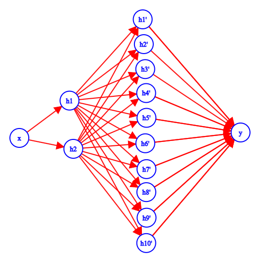
Let’s consider a simple neural network, as depicted above. Each neuron, denoted as hₖ’ in the second hidden layer, estimates a hyperplane using the following format:
hₖ’ = θ’ₖ₁h₁ + θ’ₖ₂h₂ + β₁
The equation above represents a two-dimensional hyperplane in the h₁ and h₂ space. Similarly, we can obtain the output y as follows:
y = ∑ ₀¹⁰ Ωᵢhᵢ’ + β₂
As we’ve explored in earlier blog posts, we can unfold the equation above to understand the mapping from x to y. However, our current focus is not on the specific mapping; instead, we aim to visualize how each of the ten neurons contributes to the folding process.
The neural network above is trained to estimate the following function: f(x) = sin(2x) + cos(x) + x. Each hₖ’ represents a two-dimensional surface that can be visualized. Below is a figure that illustrates the various surfaces estimated by each of the ten neurons in the second hidden layer.

Each neuron has uniquely folded the surface, providing us with insight into the various ways this folding can manifest. The latent estimation of hₖ’ in terms of x is essentially a line, which is a component of the surface depicted above. You can think of the surface as the paper on which we draw this line, and the process is akin to making cuts on the folded paper, rather than directly cutting the line itself.
Now, let’s explore how neural networks handle multiple inputs, considering a simple shallow neural network as shown in the figure below.

Instead of having just one weight at the hidden unit, we now have two weights along with a bias. With this change, each neuron estimates a plane instead of a line, while the overall mechanics remain similar. Let’s now attempt to estimate the mapping f(x₁, x₂) = sin(2x₁)sin(2x₂) + cos(x₁)cos(x₂) + x₁ + x₂ using shallow neural networks with different capacities and visualize their estimations.


As we increase the number of hidden units, our estimates of the surface we’re trying to model continue to improve. With each neuron estimating a plane, the ReLU function can cut these planes on any of their four sides, creating piece-wise linear surfaces. As mentioned earlier, the more pieces we have, the better we can approximate the target function. It’s important to note that the estimated surface is strictly piece-wise linear, even though it might give the impression of a non-linear surface. If we zoom in enough, we would clearly see these piece-wise linear regions.
Having understood how multi-dimensional inputs are handled, there’s no limitation preventing us from using deep neural networks for such estimations. Deep networks can create more of these linear regions compared to shallow networks with the same number of neurons. For instance, if we consider a 100-neuron shallow network and a deep network with two layers, each containing 50 neurons, the deep network has more parameters between the two hidden layers alone than the entire shallow network. Although both networks have the same number of neurons, we gain additional estimation power at the cost of more parameters.
The figure below shows the same estimation done by a deep network with 6 neurons in each hidden layer, and we can observe that the estimate is as good as the one obtained with a shallow neural network having 32 neurons

Let’s continue our exploration of how neural networks estimate multidimensional outputs. To gain a better understanding, let’s consider two functions, sin(x) and cos(x), both functions of a real-valued variable x. Our objective is to simultaneously learn both of these functions from the input x. We will train a simple shallow neural network, as depicted below, to estimate y₁ and y₂. In previous examples, we estimated a function with multiple variables, but now we are estimating multiple functions.


We can observe that the estimation exhibits 4 linear regions, corresponding to the 3 cuts made by each of the 3 neurons. An interesting aspect here is that both of the estimated functions have cuts at the same points. This phenomenon occurs because the neurons in the final layer estimate linear combinations of the estimations made by the neurons in the previous layer, and these linear combinations are passed through ReLU, causing cuts to be made prior to the final estimation. Consequently, the final estimation consists of two different linear combinations of these functions, resulting in cuts at precisely the same locations for both functions

Real-life problems often involve multiple variables on both the input and output sides. The figure provided below represents a generic shallow neural network capable of taking multiple inputs and returning multiple outputs. Neural networks enable us to estimate multiple multivariate functions simultaneously, making them a remarkably powerful tool for estimating complex mathematical functions.

This blog draws significant inspiration from the book “Understanding Deep Learning” by Simon J.D. Prince (udlbook.github.io/udlbook/). In the next installments, we will delve into loss functions and loss functions are derived from maximum likelihood estimation. The code I utilized to generate the plots can be found below. If you’ve found this blog insightful, I would greatly appreciate your support by giving it a like.
Understanding-Deep-Learning/Mastering_Deep_Learning_The_Art_of_Approximating_Non_Linearities_with_Pi…
Contribute to Raagulbharatwaj/Understanding-Deep-Learning development by creating an account on GitHub.
github.com
Join thousands of data leaders on the AI newsletter. Join over 80,000 subscribers and keep up to date with the latest developments in AI. From research to projects and ideas. If you are building an AI startup, an AI-related product, or a service, we invite you to consider becoming a sponsor.
Published via Towards AI
Towards AI Academy
We Build Enterprise-Grade AI. We'll Teach You to Master It Too.
15 engineers. 100,000+ students. Towards AI Academy teaches what actually survives production.
Start free — no commitment:
→ 6-Day Agentic AI Engineering Email Guide — one practical lesson per day
→ Agents Architecture Cheatsheet — 3 years of architecture decisions in 6 pages
Our courses:
→ AI Engineering Certification — 90+ lessons from project selection to deployed product. The most comprehensive practical LLM course out there.
→ Agent Engineering Course — Hands on with production agent architectures, memory, routing, and eval frameworks — built from real enterprise engagements.
→ AI for Work — Understand, evaluate, and apply AI for complex work tasks.
Note: Article content contains the views of the contributing authors and not Towards AI.


