Machine Learning With Azure’s Free Tier

Author(s): Ranganath Venkataraman

Originally published on Towards AI.

Cloud Computing

How I Continue to Stop Relying on my CPU and Use The Cloud — up to Azure’s free tier limits.

I signed up for a free subscription with Azure after exhausting my free Udacity Nanodegree’s permitted access. The free tier gives 30 days or $200 — whichever came first — of free credits towards computes for running machine learning models. I spent these first on concluding my previous work on time series forecasting and second on the SECOM dataset, following Chapter 11 of Predictive Analytics with Microsoft Azure Machine Learning, Second Edition.

This article narrates these experiences. The original code is in this GitHub repo.

SECOM dataset

This example from page 226 of the book considers data from a semiconductor manufacturing process. Various signals are monitored to predict whether the final product fails (label of 1) or passes (label of -1).

Jupyter Notebook on my computer

I imported features and labels into Python and then removed rows with null values after observing that they comprised <1% of entries.

# Featuresdata = pd.read_csv('secom.data',sep=' ',header=None)
data.isna().sum()
data.fillna(data.mean(),inplace=True)# Labels / targetlabels = pd.read_csv('secom_labels.data',sep=' ',header=None)
labels.columns = ['Class','Time']
target = labels['Class']

Since the TPOT AutoML package combines convenient preprocessing and algorithm selection, I installed the package with pip and used it to fit given data and labels using 7-cross validation

%pip install tpot
from tpot import TPOTClassifierfrom sklearn.model_selection import StratifiedKFold
cv = StratifiedKFold(n_splits=7,shuffle=True)model = TPOTClassifier(generations=5, population_size=50, cv=cv, scoring='f1_weighted',verbosity=2, random_state=1, n_jobs=-1)
# perform the search
model.fit(data,target)
# export the best model
model.export('tpot_secom_best.py')

TPOT produced a pipeline of classifiers. After splitting data and target dataframes into training and testing, I then trained TPOT’s pipeline and evaluated performance on testing data. The code in the second box below was the output of TPOT.

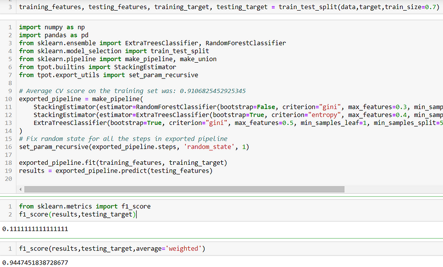
That F1-score of 0.11 is not good — interestingly the weighted F1 score is 0.94. This tells us that there’s significant space for improvement when predicting failures, a conclusion reinforced by the confusion matrix below.

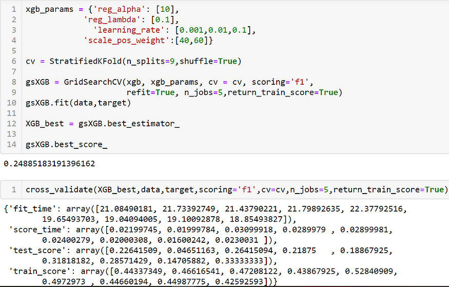
Disappointing TPOT performance drove me to try hyperparameter tuning using GridSearchCV on an XGBoost classifier that accounted for the imbalance in labels.

xgb_params = {'reg_alpha': [0.1,1,10], 
 'reg_lambda': [0.1,1,10],
 'scale_pos_weight':[7,20,40]}cv = StratifiedKFold(n_splits=9,shuffle=True)gsXGB = GridSearchCV(xgb, xgb_params, cv = cv, scoring='f1', 
 refit=True, n_jobs=5,return_train_score=True)
gsXGB.fit(data,target)XGB_best = gsXGB.best_estimator_gsXGB.best_score_

This led to a marginal improvement — an F1 score of 0.21. Tuning the learning rate further offered some more improvements based on the training and testing scores below

How does Azure ML compare with this? Let’s follow the example per page 226 of the book

Azure Designer

The book uses the Designer in Azure’s Machine Learning workspace to drag and drop datasets and modules.

This user-friendly low-code experience largely mirrors the workflow that I executed using a Jupyter notebook on my computer:

• remove missing data
• select the most salient features, as measured by Pearson correlation with the target labels. I tried anywhere from 40–50 features
• split the data with 70% used for training, the rest for test
• train boosted trees and SVMs using training data — recall that the TPOT ultimately selected a RandomForest classifier, which is also tree-based
• run hyperparameter tuning and score the best model using test data
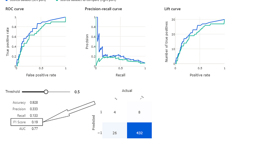
• evaluate performance using metrics of choice: I picked the F1 score, but Azure’s default appears to be the weighted score vs standard binary. Final performance was slightly below that of the full-code experience because of minor variations in hyperparameter settings.

Key take-away: this exercise and others in the book gave me some opportunities to continue trying different tools in Azure, seen next with time series forecasting.

What can be frustrating are the limits placed the power of free computes (CPUs only) in the free tier and the fact that any compute becomes off-limits after 30 days, or $200 spent. Given Microsoft’s vast resources, it’s not unreasonable to expect some marginal CPU or GPU capability on a sustained basis.

Time Series Forecasting with Azure ML notebook

The conclusion of my previous article on time series forecasting summarized the performance of various approaches including ARIMA, H2O.ai AutoML, and LSTM with/without feature extraction. Following are my observations with AzureML’s AutoML forecasting — the code used in Azure ML’s Jupyter Notebook is in this repo.

After importing the data into AzureML and doing the necessary adjustments to get a dataframe that could be manipulated (see Feature Engineering section of this article), I combined labels and features and then created a time series array.

Since the original problem in the UCI repository doesn’t state any time series, I simply used pandas datetime to create a time series array that starts on January 1, 2021 and adds a second for each row. I then called that new column ‘time’.

import datetime
base = datetime.datetime(2021, 1, 1)
arr = np.array([base + datetime.timedelta(seconds=i) for i in range(132240)])together['time'] = pd.Series(arr,index=together.index)

The time series forecasting option in Azure AutoML requires a little more work than conventional ML as outlined by the helpful Microsoft Docs. I first set forecasting parameters by identifying the ‘time’ column created earlier and setting a randomly selected forecasting horizon of 100 seconds.

from azureml.automl.core.forecasting_parameters import ForecastingParameters

forecasting_parameters_hydraulic_accum = ForecastingParameters(time_column_name='time', 
 forecast_horizon=100)

Next steps are to configure the experiment for the target variables and then actually run the experiment to observe performance. I completed these steps for hydraulic accumulation and pump leakage; see example for the latter below. I’m establishing the target metric, a timeout to prevent excessive resource usage, 5 folds for cross validation, and chose not to enable ensembling techniques — something to change in retrospect.

from azureml.train.automl import AutoMLConfig

automl_config_leak = AutoMLConfig(task='forecasting', primary_metric='normalized_mean_absolute_error',
 experiment_timeout_minutes=25,
 enable_early_stopping=True,
 training_data=together,
 label_column_name="pump_leak",
 n_cross_validations=5,
 enable_ensembling=False,
 verbosity=logging.INFO,
 forecasting_parameters=forecasting_parameters_hydraulic_accum)# Having set experiment parameters above, create workspace for running experiment.from azureml.core.experiment import Experiment
from azureml.core import Workspace

ws = Workspace.from_config()

# Choose a name for the experiment and specify the project folder.
experiment_name = 'AutoTSForecasting_hyd'
project_folder = './sample_projects/automl-classification'

experiment = Experiment(ws, experiment_name)from azureml.widgets import RunDetails

hydrun = experiment.submit(automl_config_hydraulic_accum, show_output=True)
RunDetails(hydrun).show()
hydrun.wait_for_completion(show_output=True)

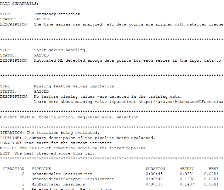
Here’s a snapshot of results for pump leakage: AutoML achieved a mean absolute error of 0.06, unable to outperform LSTM.

This exercise continues to emphasize the value of computes especially as my work demands increasingly large computing capabilities.

Join thousands of data leaders on the AI newsletter. Join over 80,000 subscribers and keep up to date with the latest developments in AI. From research to projects and ideas. If you are building an AI startup, an AI-related product, or a service, we invite you to consider becoming a sponsor.

Published via Towards AI