Logistic Regression from Scratch with Only Python Code
Last Updated on July 24, 2023 by Editorial Team
Author(s): Pushkara Sharma
Originally published on Towards AI.
Machine Learning
Applying Logistic regression to a multi-feature dataset using only Python. Step-by-step implementation coding samples in Python

In this article, we will build a logistic regression model for classifying whether a patient has diabetes or not. The main focus here is that we will only use python to build functions for reading the file, normalizing data, optimizing parameters, and more. So you will be getting in-depth knowledge of how everything from reading the file to make predictions works.
If you are new to machine learning, or not familiar with logistic regression or gradient descent, don’t worry I’ll try my best to explain these in layman’s terms. There are more tutorials out there that explain the same concepts. But what makes this tutorial unique is its short and beginners friendly high-level description of the code snippets. So, let's start by looking at some theoretical concepts that are important in order to understand the working of our model.
Logistic Regression
Logistic Regression is the entry-level supervised machine learning algorithm used for classification purposes. It is one of those algorithms that everyone should be aware of. Logistic Regression is somehow similar to linear regression but it has different cost function and prediction function(hypothesis).

Sigmoid function
It is the activation function that squeezes the output of the function in the range between 0 and 1 where values less than 0.5 represent class 0 and values greater than or equal to 0.5 represents class 1.

Cost Function
Cost function finds the error between the actual value and predicted value of our algorithm. It should be as minimum as possible. In the case of linear regression, the formula is:-

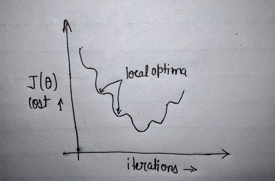
But this formula cannot be used for logistic regression because the hypothesis here is a nonconvex function that means there are chances of finding the local minima and thus avoiding the global minima. If we use the same formula then our plot will look like this:-

So, in order to avoid this, we have smoothened the curve with the help of log and our cost function will look like this:-

where m=number of examples or rows in the dataset, xᶦ=feature values of iᵗʰ example, yᶦ=actual outcome of iᵗʰ example. After using this, our plot for the cost function will look like this:-

Gradient Descent
Our aim in any ML algorithm is to find the set of parameters that minimizes the cost function. And for automatically finding the best set of parameters we use optimization techniques. One of them is gradient descent. In this, we start with random values of parameters(in most cases zero) and then keep changing the parameters to reduce J(θ₀,θ₁) or cost function until we end up at a minimum. The formula for the same is:-

It looks exactly the same as that of linear regression but the difference is of the hypothesis(hθ(x)) as it uses sigmoid function as well.
That’s a lot of theory, I know but that was required to understand the following code snippets. And I have only scratched the surface, so please google the above topics for in-depth knowledge.
Prerequisites:
I assume that you are familiar with python and already have installed the python 3 in your systems. I have used a jupyter notebook for this tutorial. You can use the IDE of your like. All required libraries come inbuilt in anaconda suite.
Let’s Code
Okay, so I have imported CSV, numpy(for majorly dot product only), and math for performing log and exponential calculations.
Read the File
Firstly, we have defined the function read_filefor reading the dataset itself. Here, the file is opened with with so we don't have to close it and stored it in the reader variable. Then we loop over reader and append each line in the list named dataset. But the loaded data is of string format as shown in screenshot below.

Convert String to Float
The string_to_float function here helps to convert all string values to float in order to perform calculations on it. We simply loop on each row and column and convert every entry from string to float.

Find Min Max
Now, in order to perform normalization or getting all values on the same scale, we have to find the minimum and maximum values from each column. Here in function, we have loop column-wise and append the max and min of every column in minmax list. Obtained values are shown in the screenshot below.

Normalization
Now, we have looped over every value in the dataset and subtract minimum value (of that column) from it and divide it with the difference of max and min of that column. The screenshot below represents the normalized values of a single row example.

Train Test Split
Here, train_test function helps to create training and testing datasets. We have used shuffle from random module to shuffle the whole dataset. Then we slice the dataset to 80% and store it in train_data and the remaining 20% in test_data . The size of both sets is shown below.

Accuracy
This accuracy_check function will be used to check the accuracy of our model. Here, we simply looped over the length of the actual or predicted list as both are of the same length and if the value at the current index of both are same, we increase the count c . Then just divide that count c with the length of the actual or predicted list and multiply by 100 to get the accuracy %.
Prediction or Hypothesis Function
Yes, here we have imported numpy to calculate dot product but function for that can also be made. math for calculating exponential. The prediction function is our hypothesis function that takes the whole row and parameters as arguments. We have then initialized hypothesis variable with θo and we looped over every row element ignoring the last as it is the target y variable and added xᵢ*θ(i+1) (i+1 is in subscript) to hypothesis variable. After that, comes the sigmoid function 1/(1+exp(-hypothesis)) that squeezes the value in the range of 0–1.
Cost Function
We don’t necessarily need this function to get our model worked but it is good to calculate the cost with every iteration and plot that. Incost_function we have looped over every row in the dataset and calculated costof that row with the formula described above then add it to the cost variable. Finally, the average cost is returned.
Optimization Technique
Here, we have used gradient_descent for automatically finding the best set of parameters for our model. This function takes dataset, epochs(number of iterations), and alpha(learning rate) as arguments. In the function, cost_history is initialized to append the cost after every epoch and parametersto hold the set of parameters(no. of paramters=features+1). After that, we started a loop to repeat the process of finding the parameters. The inner loop is used to iterate over every row in the dataset. Here gradient term is different for θo due to partial derivative of the cost function, that's why it is calculated separately and added to 0th position in parameters list, then other parameters are calculated using other feature values of row(ignoring last target value) and added to their respective position in the parameters list. The same process repeats for every row. After that 1 epoch is completed and cost_function is called with the calculated set of parameters and the value obtained is appended to cost_history .
Combining Algorithm
Here, we have imported matplotlib.pyplot just to draw the cost plot. So it is not necessary. In algorithm function, we are calling the gradient_descent with epochs=1000 and learning_rate = 0.001. After that, making predictions on our testing dataset. round is used to round off the obtained predicted values(i.e. 0.7=1,0.3=0). Then, accuracy_check is called to get the accuracy of the model. At last, we have plotted the iterations v/s cost plot.
Putting Everything Together
Just to have a proper structure, we have put all the functions in a single combine function. We were able to achieve an accuracy of around 78.5% which can be further improved by hyper tuning the model. The plot below also proves that our model is working correctly as cost is decreasing with an increase in the number of iterations.

Conclusion
We have successfully build a Logistic Regression model from scratch without using pandas, scikit learn libraries. We have achieved an accuracy of around 78.5% which can be further improved. Also, we can leave numpy and built a function for calculating dot products. Although we will use sklearn, it good to know the inner working as well. U+1F609
The source code is available on GitHub. Please feel free to make improvements.
Thank you for your precious time.U+1F60AAnd I hope you like this tutorial.
Also, check my tutorial on a Gradient Descent v/s Normal Equation
Gradient Descent v/s Normal Equation For Regression Problems
Choosing the right algorithm to find the parameters that minimize the cost function.
medium.com
Simple Text Summarizer Using Extractive Method
Automatically makes a small summary of the article containing the most important sentences.
towardsdatascience.com
Join thousands of data leaders on the AI newsletter. Join over 80,000 subscribers and keep up to date with the latest developments in AI. From research to projects and ideas. If you are building an AI startup, an AI-related product, or a service, we invite you to consider becoming a sponsor.
Published via Towards AI
Towards AI Academy
We Build Enterprise-Grade AI. We'll Teach You to Master It Too.
15 engineers. 100,000+ students. Towards AI Academy teaches what actually survives production.
Start free — no commitment:
→ 6-Day Agentic AI Engineering Email Guide — one practical lesson per day
→ Agents Architecture Cheatsheet — 3 years of architecture decisions in 6 pages
Our courses:
→ AI Engineering Certification — 90+ lessons from project selection to deployed product. The most comprehensive practical LLM course out there.
→ Agent Engineering Course — Hands on with production agent architectures, memory, routing, and eval frameworks — built from real enterprise engagements.
→ AI for Work — Understand, evaluate, and apply AI for complex work tasks.
Note: Article content contains the views of the contributing authors and not Towards AI.


