Logistic Regression Explained

Author(s): Jin Cui

Originally published on Towards AI the World’s Leading AI and Technology News and Media Company. If you are building an AI-related product or service, we invite you to consider becoming an AI sponsor. At Towards AI, we help scale AI and technology startups. Let us help you unleash your technology to the masses.

A practitioner’s guide

Logistic Regression for Classification Problems

Logistic Regression is known for modeling classification problems. I’ll demonstrate the advantages of using a Logistic Regression over a Linear Regression for a classification problem with an example.

In the insurance context, a lapse refers to the event that a policyholder exercises the option to terminate the insurance contract with the insurer. It’s in the insurer’s interest to understand whether a policyholder is likely to lapse at the next policy renewal, as this typically helps the insurer prioritize its retention efforts. This then becomes a classification problem as the response variable takes the binary form of 0 (non-lapse) or 1 (lapse), given the attributes of a particular policyholder.

In the synthetic dataset underlying the chart below, we record the lapse behavior of 30 policyholders, with 1 denoting a lapse and 0 otherwise. It can be observed that there is a strong non-linear relationship between the probability of lapse and policyholder’s age. In particular, it appears that lapses are mostly associated with ages greater than 50.

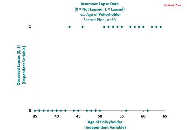
Chart 1: Observed lapses of 30 policyholders. Chart by author

It would be counter-intuitive to model lapses in this instance using Linear Regression as indicated by the grey line in the chart below. Instead, a Logistic Regression as indicated by the green line provides a better fit.

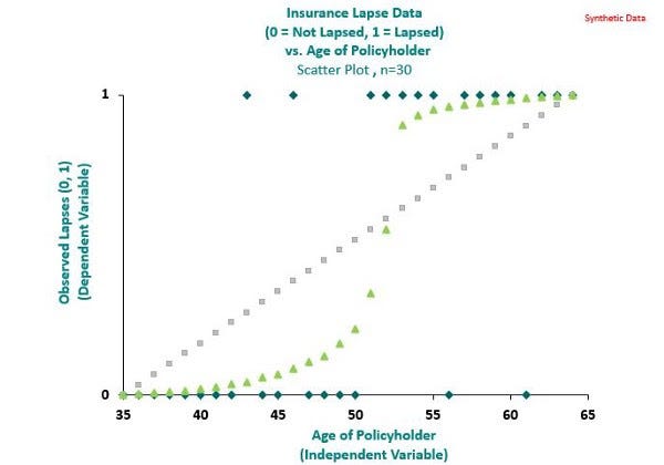
Chart 2: Linear Regression vs. Logistic Regression. Chart by author

Logistic Regression belongs to the family of Generalised Linear Models (“GLM”), which are commonly used to set premium rates for General Insurance products such as motor insurance. Assuming we want to model the probability of lapse for a policyholder denoted by p, a Logistic Regression has a variance function in the form of the below, which is minimized when p takes the value of 0 or 1.

This is a nice attribute for modeling the probability of lapse for a policyholder as the observed lapse takes the value of 0 or 1. An accomodating consequence of this is that the Logistic Regression gives greater credibility to observations of 0 and 1 as shown by the green line in Chart 2. This makes Logistic Regression suitable for modeling binary events such as predicting whether a policyholder will lapse, or whether a transaction is fraudulent, which is easily extendable to other classification problems.

The Log-odds Ratio

Predictive models aim to express the relationship between the independent variable(s) (“X”) and the dependent variable (“Y”). In a Linear Regression, the relationship may be expressed as:

In this instance, Y may represent the property price, and X₁ and X₂ may represent the property size and number of bedrooms in the property respectively, in which case we would expect a positive relationship between the independent and dependent variables in the form of positive coefficients for β₁ and β₂.

To model the probability of lapse for a policyholder (“p”), we modify equation (2) slightly by replacing the Y with the Log-odds Ratio below:

In simple terms, if the probability of lapse for a particular policyholder is 80%, which implies the probability of non-lapse is 20%, then the term inside the bracket in equation (3) is 4. That is, this policyholder is 4 times more likely to lapse than not lapse, or the odds ratio is 4. The Log-odds Ratio further scales this with the log operation.

Mathematically, equation (3) can be written in other forms such as equations (4) and (5) below:

After the β coefficients are estimated under the Logistic Regression, equations (4) and (5) make interpretation of the Logistic Regression model outputs comprehensive for the following reasons:

• Equation (4) expresses the odds ratio using a structure that maintains linearity.
• Equation (5) maps the features to a probability ranging from 0 to 1. This enables users of the model to allocate a probability of lapse to each policyholder, from which retention efforts can be prioritized quantitatively.

In addition, by having an intercept term β₀, a baseline scenario is easily established for benchmarking. To explain this using a simple example, assume that X₁ denotes the gender of the policyholder (i.e. a categorical variable of two levels — Male or Female) and X₂ denotes the income level of the policyholder (i.e. another categorical variable of two levels — High or Low), with the response variable still being the probability of lapse. The baseline scenario can be set up to represent a male policyholder with a low-income level with the proper encoding of the said categorical variables. Using equation (4), β₁ and β₂ then represent step-change in odds ratio to the baseline scenario by quantum the respective coefficients.

To demonstrate, to understand the effect of income level on the probability of lapse:

Equation (6) implies that the effect on the probability of lapse by income level is a constant based on coefficient β₂.

The Coefficients

It can be inferred from equation (6) that the sign of the β coefficients show the direction in which the corresponding features (in this instance, the income level) influence the odds ratio and that the quantum or size of the β coefficients show the extent to which the features influence the odds ratio.

However, in practice, not all features are reliable, as their corresponding β coefficients are not statistically significant. As a rule of thumb, features typically are considered significant with a p-value less than 0.05, suggesting that these β coefficients have relatively small variance, or that the value as defined below is high.

β coefficients of large variance indicate that less reliance should be placed on the corresponding feature, as the estimated coefficients may vary over a wide range.

Multivariate Analysis

Using the p-value, Logistic Regression (although not restricted to Logistic Regression) is able to filter out non-significant features which may be highly correlated with other existing features. This helps identify the true underlying drivers of an event we are trying to predict.

By way of example, the sum insured of a policy and the income of a policyholder may be highly correlated due to financial underwriting. A relationship may have been observed between high lapses and policyholders with low sums insured, how can we be certain that the underlying lapses are not driven by the income levels instead?

Logistic Regression handles this by allocating a high p-value for ‘expendable’ features which can be replaced by including other existing features. Using the same example, if the low-income level were the true driver of lapses, the model is invariant between high and low sums insured, in that although low sums insured predicted lapses for some instances, the model is still predictive when this feature is switched off and low-income level is used (i.e. the sum insured feature has higher variance).

Limitations

There are some known limitations of applying Logistic Regression (or more generally, GLM) in practice, including:

• It requires significant feature engineering effort as features may need to be manually fitted. This includes the fitting of interaction terms where the effect of one feature may depend on the level of another feature. One example of this interaction in the insurance context is the premium increases may differ by age. The number of possible interaction terms increases exponentially with the number of features. In addition, although Logistic Regression allows investigation into interaction terms, they may prove difficult to interpret.
• The independent variables (X) are by assumption independent, which may not be true. For the use case of predicting lapses, the lapse events may need to be measured and segmented by time periods (as all policies would have lapsed over time), which may introduce overlapped policies in different periods and result in correlations.

Summary

In conclusion, Logistic Regression provides a reasonable baseline model for classification problems, as it adjusts for correlation between features and allows for comprehensive model interpretation. In practice, it is in a practitioner’s best interest to compare the performance of the Logistic Regression model against other models known for solving classification problems (such as tree-based models) for best inferences.

Like what you are reading? Feel free to visit my Medium profile for more!

Logistic Regression Explained was originally published in Towards AI on Medium, where people are continuing the conversation by highlighting and responding to this story.

Join thousands of data leaders on the AI newsletter. It’s free, we don’t spam, and we never share your email address. Keep up to date with the latest work in AI. From research to projects and ideas. If you are building an AI startup, an AI-related product, or a service, we invite you to consider becoming a sponsor.

Published via Towards AI