


LogBERT Explained In Depth: Part I
Last Updated on September 26, 2022 by Editorial Team
Author(s): David Schiff
Originally published on Towards AI the World’s Leading AI and Technology News and Media Company. If you are building an AI-related product or service, we invite you to consider becoming an AI sponsor. At Towards AI, we help scale AI and technology startups. Let us help you unleash your technology to the masses.
One of the greatest frontiers in IT and system administration is dealing with application and system failures. Sometimes the reason for the failure is extremely difficult to find. When system technicians and application developers need to find the cause for the failure of their application, they usually read the log files generated by said system. The technician will then find the log relevant to the crash and will use this information to recover from the failure. The problem with this technique is that sometimes systems and applications generate hundreds of thousands of logs and even millions. The job of looking for the single log message that would have predicted the crash could take a very long time, and the task itself may be exhausting.
Over the years, many methods have been proposed for dealing with this task of finding the relevant log message. Many of these methods use ideas that come from the anomaly detection field. As we can assume a priori, the log that will predict the crash and can give an indication as to what caused it should itself be anomalous. This is because if it was not anomalous, we could not tell the difference between normal system activity and activity that could predict an upcoming failure.
Anomaly detection as it is, up until recently, had mostly involved different feature extraction techniques implemented for usage in classic anomalies detection models such as IsolationForest or OneClassSVM and many more. The idea is basically that we extract relevant features from the text that could be relevant for discriminating between normal and anomalous logs. The problem with this technique is that we assume many things about the distribution of our data. Moreover, this technique is not as general as we would like it to be. One feature extraction technique could be relevant for HDFS logs, and another would be relevant for SQL logs. This means that there is no “universal model” for log anomaly detection.
Lately, techniques that involve deep learning have become popular. Using Recurrent Neural Networks such as LSTM or GRU has been a popular method for detecting anomalies in sequences such as the text sequences that are present in system logs. Unfortunately, RNNs lack the memory we need for a complex analysis of system logs.
In this article, I would like to explain and simplify the LogBERT method for detecting anomalies in log sequences.
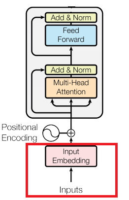
To start the in-depth analysis, we will break down the transformer block, which is the main component of BERT.
To start off, we’ll get into the embedding layer. An important component in most neural networks dealing with natural language. So how does an embedding layer work?
Embeddings — word embeddings, to be precise, are representations of tokens in some vector space. We would like these vector representations to capture the meaning of the word itself. A great example of a type of word embedding method is Word2Vec. The goal of Word2Vec is to maximize the cosine similarity of the word embeddings that appear in the same context in a sentence [I really like eating apples. I enjoy eating tuna. => tuna and apples should have similar representations]. We won’t get into that here, but you get the idea. The goal is to find some representation of a word that would be meaningful enough when given as input to a neural network.
So how do we process a sentence into something meaningful? In our case, how do we process a sequence of words in a log message into something meaningful? Let’s dive into it.
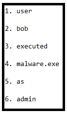
Well, start with a running example we’ll use throughout our series of articles.

We would start by tokenizing this sentence, each word would be considered a token. We then end up having a token list. Of course, in a log file, there are many more words but just consider this single log message for the example. Each word will be placed in a dictionary or a list with a number representing it as such (I’m not getting rid of all the stop words and doing other preprocessing steps just for this example):
Now, the embedding layer looks like this:
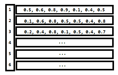
What we see here is an array containing vectors in each cell of the array. Essentially what happens is that when a sequence of words [1,2,3,4,5,6] is given as input to the neural network, the embedding layer translates each word index to a vector representation using the embedding layer. So the neural network itself does not see a sequence of words nor a sequence of indexes but a sequence of vectors! The embedding layer itself has a configurable embedding size (the dimension of a word representation). Just for fun, another example would be:
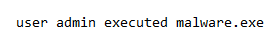
This would be translated to the sequence [1,6,3,4], which would mean our embedding layer takes the vector in index no. 1 in the embedding matrix, then vector no. 6, and then no. 3 and finally, no. 4. Of course, padding will be necessary since we should have a constant length in our sequences. And the result will be a matrix that represents our sentence or sequence.
Now that we got it, let's sum it up:
The embedding layer contains an embedding matrix which basically contains a reference to a vector that should represent that word. When words are fed into the embedding layer, they are fed as sequences of indexes referring to the vectors that should represent them in the embedding matrix.
Mathematically, it can be represented as the matrix multiplication of two matrices. Matrix A is the one-hot vector representation of the words in the sentence, and Matrix B is the embedding matrix itself containing the vector representations of each word in the corpus. So A x B Should give us the full sequence of words represented as vectors.
The next part of the transformer block is position encoding. This is the part of the transformer block where we encode the information about the position of the word in the sequence. How is this done?
Given a vector V = <a,b,c,d>, which represents the embedding of some word X we would like to represent the word position in the sequence itself.
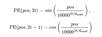
As we can see, this function is used to encode the position of a word. How is this done? Given a word sequence, the word X could be present in different positions in the sequence. Say, in an instance of a sentence, the word could be positioned in the middle as such:
Bob ate two X this morning.
In this case, X is in the middle of the sentence, and the position of X is 4 and will be encoded using the function above. If V is embedded in a 4 dimensional space as stated above V = <a,b,c,d> then the transformation of V will be:
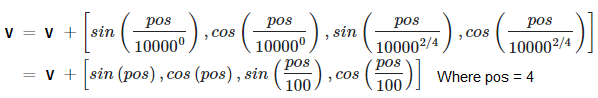
And then finally, we have our word X represented in 4-dimensional space using our embedding layer and the position encoding layer to capture the locations of the word in the sequence.
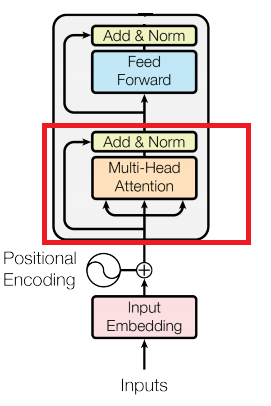
Next, our sequence, represented as a DxN dimensional matrix where D represents our embedding dimensions and N represents our sequence size, is fed into the multi-head attention layer. Let's dive into it.
What is multi-head attention? Let's start with a simple self-attention layer:
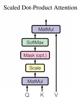
Essentially, Self Attention is a function that we perform on our input matrix:
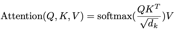
We are going to break this function down, but for this article, we will ignore the denominator as it is used for normalization and is not core to understanding the idea behind the attention.
We have our self-attention over here. The process is comprised of a few stages. The first is we apply a linear transformation on our input matrix 3 times — one for the Query matrix, another for the Key, and another for the Value (We’ll call them Q,K,V). Again, our input matrix is essentially the input sequence encoded as vectors. So our input matrix is being transformed into three different matrices.
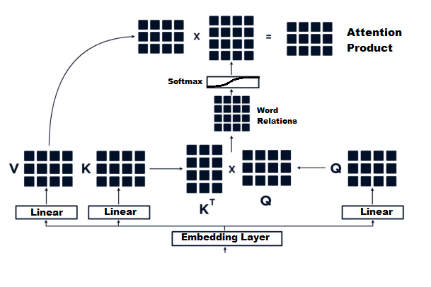
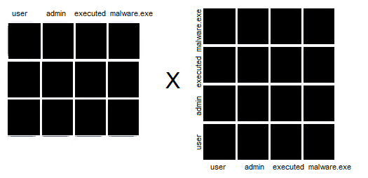
In the picture above, we can see that matrix multiplication is applied to the Key and Value matrix. This results in a matrix that represents our bi-directional word relations (of course, after the weights in the matrices are learned properly). This word relations matrix allows us to capture the structure and the meaning of the sentence in a way that we haven’t been able to capture in the previous sequence learning neural networks such as LSTM or GRU. This is because those types of neural networks suffer from a lack of long-term memory, while self-attention attends to relations between words all throughout the sentence like so:
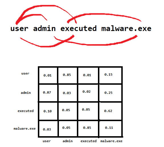
The attention matrix, which captures the word relations, is finally multiplied by the value matrix. Notice how each word has a “score” as to how much it is related to other words in the sentence. In the above example, the user and admin have a high relation score.
As mentioned in the paper (Neural Machine Translation by Jointly Learning to Align and Translate), attention, by definition, is just a weighted average of values,
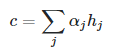
where

If we restrict α to be a one-hot vector, this operation becomes the same as retrieving from a set of elements h with index α. With the restriction removed, the attention operation can be thought of as doing “proportional retrieval” according to the probability vector α.
It should be clear that h in this context is the value (in our case, the value matrix).
After noting this, we can see that the value matrix is multiplied by the matrix resulting from multiplying the query and the key. This ends up being the exact definition of attention, as we were using a weighted retrieval technique with the weights α being drawn from the word relations matrix.
If we apply matrix multiplication here, we’ll see that the encoding for a sequence in the matrix on the left is multiplied by the proportional relation of each word to all the other ones.
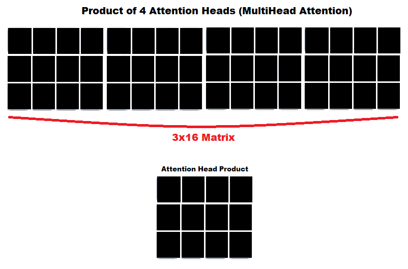
Next, we have Multi-Head Attention. This is similar to the multiple filters we use in convolutional neural networks. The reason is that we use multiple filters to capture different patterns in our picture that could indicate whatever we are looking for in that picture. In Multi-Head Attention, we capture different possible relations in the sentence that could result in different meanings altogether. Multi-Head Attention is actually very simple once we get the hang of attention. Essentially, all we do is concatenate the resulting matrices of the attention heads like so:
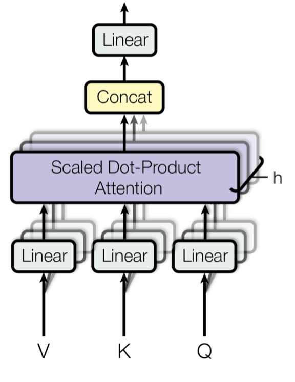
Concatenation means we just attach all the matrices to each other. The final product should be a large matrix.
This part should have summed up the main components of the LogBERT and the BERT Structure. I didn’t get into all the normalization layers and scaling and all that because I thought it was not much of a key detail and didn’t want to waste time writing about it. If anyone is confused about it, they can read up about it somewhere else.
In the next part, I want to cover the final LogBERT architecture and loss function so we can see how it all fits together. Thanks for reading so far.
LogBERT Explained In Depth: Part I was originally published in Towards AI on Medium, where people are continuing the conversation by highlighting and responding to this story.
Join thousands of data leaders on the AI newsletter. It’s free, we don’t spam, and we never share your email address. Keep up to date with the latest work in AI. From research to projects and ideas. If you are building an AI startup, an AI-related product, or a service, we invite you to consider becoming a sponsor.
Published via Towards AI
Towards AI Academy
We Build Enterprise-Grade AI. We'll Teach You to Master It Too.
15 engineers. 100,000+ students. Towards AI Academy teaches what actually survives production.
Start free — no commitment:
→ 6-Day Agentic AI Engineering Email Guide — one practical lesson per day
→ Agents Architecture Cheatsheet — 3 years of architecture decisions in 6 pages
Our courses:
→ AI Engineering Certification — 90+ lessons from project selection to deployed product. The most comprehensive practical LLM course out there.
→ Agent Engineering Course — Hands on with production agent architectures, memory, routing, and eval frameworks — built from real enterprise engagements.
→ AI for Work — Understand, evaluate, and apply AI for complex work tasks.
Note: Article content contains the views of the contributing authors and not Towards AI.
Related posts
Recent Posts


")

