Half Marathon Data Exploration and Visualization: using Python Plotly Library

Author(s): David Cullen

Originally published on Towards AI.

London Landmarks Half Marathon 2023

In April of this year, I ran the London Landmarks Half Marathon for the first time. The race included 17,225 registered participants between the ages of 17–89 and managed to raise over £10 million for 450 charities (well-done everyone!).

Following the race, I was emailed helpful summary statistics, such as position in the race, average speed, and split times, including a link to the race data in.xlsx format.

In addition to the summary statistics already available, I thought it would be interesting to explore the data in a bit more detail, which led me to write this article, covering:

• Data Extraction: download data and store it in Pandas DataFrame.
• Data Preparation: data cleaning using NumPy and Pandas.
• Data Overview: data overview, visualized using Plotly.
• Data Distribution: kernel density estimation and empirical cumulative distribution function visualized using Plotly.
• Average Speed Analysis: analysis of participant speed across a variety of chiptime splits, visualized using Plotly.

Each analysis in this article includes the relevant Python code to enable the reader to follow along programmatically.

Important Note: The majority of the visuals in this article are interactive — just follow the link in each respective title. For this, I have used Plotly Chart Studio: https://chart-studio.plotly.com. A tutorial on implementing interactive plots is outside the scope of this article. The reader will be able to replicate the visuals in this article directly from their interactive computing environment (i.e., Jupyter Notebook).

Dataset

The dataset [1] consists of 26 attributes, of which the following has been used in this article:

• Chiptime: Finishing chiptime.
• Category: Age group by gender.
• Gender: Male or Female.
• Avg speed: Runner km/hr average race speed.
• Split — 5K — Cumulative time: Runner 5k time.
• Split — 10K — Cumulative time: Runner 10k time.
• Split — 15K — Cumulative time: Runner 15k time.
• Split — 20K — Cumulative time: Runner 20k time.

I chose the above attributes, as I personally have found these data most interesting from a performance perspective.

Below details the process for data extraction.

Import Libraries:

We will first import the required libraries:

import requests # html requests
import numpy as np # data analysis
import pandas as pd # dataframe creation and analysis
from scipy import stats # central tendency anaysis
import dash # plots
import jupyter_dash # open plots in notebook
import plotly.express as px # plots 
import plotly.figure_factory as ff # plots
import locale # comma separators in plot

Data Extraction:

We will now inspect the link html and find the relevant href. From here we extract the url to get the required data.

# url 
url = "https://mel-active-eventresults-webdynamiccontent.azurewebsites.net/data/downloadexcel?eventId=7037394564091167232&raceId=485022" # href url to dataset

# open the .xlsx file
with open('LLHM2023.xlsx', 'wb') as out_file:
 response = requests.get(url, stream=True) # get data
 content = response.content # get content
 out_file.write(content) # write content 

# dataframe 
df = pd.read_excel('LLHM2023.xlsx').fillna(0) # create dataframe and fill na with 0
df1 = (df[['Chiptime','Split - 5K - Cumulative time','Split - 10K - Cumulative time','Split - 15K - Cumulative time','Split - 20K - Cumulative time','Gender','Avg speed','Category']])# create dataframe for analysis, selecting specific attributes.
df1.head() # inspect first 5 rows of the data

By running the above code, the data should now have been successfully stored in a DataFrame (df1) for cleansing.

Data Preparation:

We will now clean df1 to make it a bit more workable:

Datetime columns:

• Convert time objects to second integers for later analysis.
• Remove data that does not indicate Chiptime, to include recorded completion times only.

Category Column:

• Convert Category elements to a sortable format for later analysis (i.e. remove gender prefix).

Gender Column:

• Convert Gender elements to a readable format (from m and f to Male and Female).
• Remove entries that do not specify the participant’s gender.

Average Speed Column:

• Round the average speed for each participant to 2 decimal places.

General Column Renaming:

• Rename columns to a clearer format.

The following function has been used to complete the above:

def clean_dataset(data):
 
 # format time related columns
 data['Chiptime Seconds'] = pd.TimedeltaIndex(data['Chiptime'].astype("str")).total_seconds().astype(int) # create seconds column
 data = data[data['Chiptime Seconds'] > 0] # remove 0 value rows to only show registered completed particpants
 data.loc[:, 'Split - 20K - Cumulative time'] = pd.TimedeltaIndex(data['Split - 20K - Cumulative time'].astype("str")).total_seconds().astype(int) # convert to seconds
 data.loc[:, 'Split - 10K - Cumulative time'] = pd.TimedeltaIndex(data['Split - 10K - Cumulative time'].astype("str")).total_seconds().astype(int)# convert to seconds
 data.loc[:, 'Split - 15K - Cumulative time'] = pd.TimedeltaIndex(data['Split - 15K - Cumulative time'].astype("str")).total_seconds().astype(int) # convert to seconds
 data.loc[:, 'Split - 5K - Cumulative time'] = pd.TimedeltaIndex(data['Split - 5K - Cumulative time'].astype("str")).total_seconds().astype(int) # convert to seconds
 
 # format 'Category' column
 data['Category'] = data['Category'].str.slice(1)# slice first character (M/F), to enable category sorting of age category.
 data.sort_values(by='Category', inplace=True) # category sorting 
 data['Category'].replace({'BC': 'Unknown'}, inplace=True) # preprocess 
 data = data[data['Category'] != 'Unknown'] # drop Unknown 
 
 # format "Gender" column
 data["Gender"].replace(to_replace = "m",value="Male", inplace = True) # replace elemments in Gender column
 data["Gender"].replace(to_replace = "f",value="Female", inplace = True) # replace elemments in Gender column
 data["Gender"].replace(to_replace = 0,value="Not Specifed", inplace = True) # replace elemments in Gender column
 data = data[data['Gender'] != 'Not Specifed'] # drop not specifed 
 
 # format 'Avg speed' column
 data['Avg speed'] = data['Avg speed'].round(2) # round average speed
 
 # general column renaming
 data = data.rename(columns = {'Avg speed':'Avg speed km/hr','Category':'Age Category'}) # rename specified columns 
 
 return data

# clean and show the data
cleaned_df = clean_dataset(df1)
cleaned_df 

Data Overview:

Now we can inspect the cleansed data.

Participants by Gender and Age Category:

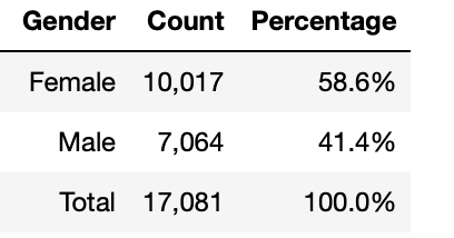
Following data cleaning, 17,081 participant entries are usable. From this total, the majority of the participants were female, making up 58.6%. The remaining 41.4% of participants were male.

# calculate count and percentage of each 'Gender'
gender = cleaned_df.groupby(['Gender']).size().reset_index()
gender = gender.rename(columns={0: 'Count'})
gender['Percentage'] = gender.groupby(['Gender']).apply(lambda x: 100 * x / gender['Count'].sum()).round(1)

# add total row
total_row = gender[['Count']].sum().rename({0: 'Total'})
total_row['Percentage'] = (total_row['Count'] / total_row['Count'].sum() * 100).round(1)
gender = pd.concat([gender, total_row.to_frame().T])

# format percentage column elements
gender['Percentage'] = gender['Percentage'].astype(str) + '%'

# format count column elements
gender['Count'] = gender['Count'].map('{:,.0f}'.format)
gender = gender.reset_index()
gender = gender.drop(columns=['index'])
gender.loc[gender.index[-1], 'Gender'] = 'Total'

# show
gender

Count and Percentage of Participants by Age Category — Bar Chart:

Figure 1 shows the count and percentage of participants by age category across males and females.

25–29 is the most common age category, with 2,948 participants. This is then followed by age categories 30–34, totaling 2,434 participants, and 40–44, totaling 2,410 participants.

Less common age categories are 17–19, which sees 189 participants, and 65–69, which sees 153 participants. A substantial reduction in participants can also be seen from age 70 on.

# create percentage by 'Age Category' dataframe
perc_age_group = cleaned_df.groupby(["Age Category"]).size().reset_index() # group by 'Age Category'
perc_age_group['Percentage'] = cleaned_df.groupby(["Age Category"]).size().groupby(level=0).apply(
 lambda x: x / perc_age_group[0].sum()).values.round(4) *100 # add percentage column


# create a new column with concatenated values of 'Count' and 'Percentage' rounded to 2decimal place
perc_age_group.rename(columns = {0: 'Count'}, inplace = True)
perc_age_group['Count and Perc'] = perc_age_group['Count'].astype(str) + ' U+007C ' + perc_age_group['Percentage'].round(2).astype(str)+'%'

# set the locale for comma separators
locale.setlocale(locale.LC_ALL, '')

# create a new column with separate lines for 'Count' and 'Percentage'
perc_age_group['Text'] = (
 perc_age_group['Count'].apply(lambda x: locale.format_string("%d", x, grouping=True)) + '<br>' +
 perc_age_group['Percentage'].round(2).astype(str) + '%'
)
# plot 
fig = px.bar(
 perc_age_group,
 x="Age Category",
 y="Percentage",
 text="Text",
 template="simple_white"
)
# update traces 
fig.update_traces(
 textposition="outside",
 textfont=dict(size=12) 
)
# set plot colors and bar width
fig.update_traces(marker_color='grey')
fig.update_traces(width=0.90)

# set y-axis tick suffix as percentage
fig.update_layout(yaxis_ticksuffix='%')

# set y-axis range
fig.update_layout(yaxis_range=[0, 20])

# show
fig.show()

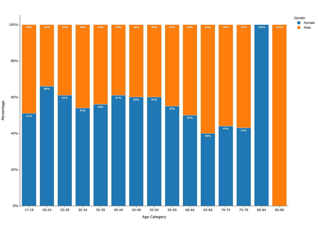
Percentage of Male and Female Participants by Age Category — Stacked Bar Chart:

Figure 2 shows that female participants represent the majority in most age categories.

# percentage of 'Male' and 'Female' participants by 'Age Category':
perc_by_gender_and_age=cleaned_df.groupby(["Age Category","Gender"]).size().reset_index() # group 
perc_by_gender_and_age['Percentage'] = cleaned_df.groupby(["Age Category","Gender"]).size().groupby(level=0).apply(lambda 
 x:100 * x/float(x.sum())).values.round(0) # add percentage of 'Gender'

# plot 
fig=px.bar(perc_by_gender_and_age, x='Age Category', y='Percentage',color='Gender',text='Percentage',template="simple_white",text_auto=True)

# update layout 
fig.update_layout(yaxis_ticksuffix = "%") 

# update traces
fig.update_traces (textfont=dict(size=10,color='white')) 
# show
fig.show()

Data Distribution:

Chiptime Kernel Density Estimation:

We will now perform Kernel Density Estimation (KDE) on the chiptime for all participants to estimate the probability density function. This will give us a good indication of the distribution of the data.

As shown, the distribution is right-skewed. The mode (most common value) and median (central value) are less than the mean (average). This is a characteristic of a right-skewed distribution due to the large spread in the right tail, representing slower half marathon chiptimes.

Inspection of the mean indicates an average completion time of 2 hours, 15 minutes. An increasing number of participants took longer to complete the race, as indicated by the elongated right tail, which pulls the average (mean) completion time upwards.

Following the examination of the median and mode, a different picture emerges. For example, 50% of all runners ran the race in 2 hours, 10 minutes, or less (median), and the most frequent participation completion time was 1 hour, 57 minutes (mode).

# create dataframe for plot
hist_data = [cleaned_df['Chiptime Seconds']]
group_labels = ['Density'] # group 
colors = ['#333F44'] # colour 

# create distplot
fig = ff.create_distplot(hist_data, group_labels,colors=colors,curve_type='kde',show_hist=False,show_curve = True) # kde plot

# calculate the mean, mode and median based on 'Chiptime' seconds
mean_chiptime = np.mean(cleaned_df['Chiptime Seconds'])
mode_chiptime = stats.mode(cleaned_df['Chiptime Seconds'])
median_chiptime = np.median(cleaned_df['Chiptime Seconds'])

# mean, mode and median as datetime object 
mean_chiptime_text = pd.to_datetime(mean_chiptime, unit='s').strftime('%H:%M:%S')
mode_chiptime_text = pd.to_datetime(mode_chiptime[0].item(), unit='s').strftime('%H:%M:%S')
median_chiptime_text = pd.to_datetime(median_chiptime, unit='s').strftime('%H:%M:%S')

# add a vertical line for the mean, mode and median on plot
fig.add_vline(x=mean_chiptime, line_color='red', line_dash='dot',annotation_text= (f'Mean:{mean_chiptime_text}'),annotation_font=dict(color='red'))
fig.add_vline(x=mode_chiptime[0].item(), line_color='blue', line_dash='dot', annotation_text= (f'Mode:{mode_chiptime_text}'),annotation_position="top left",annotation_font=dict(color='blue'))
fig.add_vline(x=median_chiptime, line_color='yellow', line_dash='dot', annotation_text= (f'Median:{median_chiptime_text}'),annotation_position="bottom right",annotation_font=dict(color='yellow'))

# add datetime to x axis 
fig.update_xaxes(
 title='Chiptime',
 showline=True,
 tickvals=list(range(0, int(cleaned_df['Chiptime Seconds'].max()) + 5, 800)),
 ticktext=pd.to_datetime(list(range(0, int(cleaned_df['Chiptime Seconds'].max()) + 5, 800)), unit='s').strftime('%H:%M:%S'),
 tickangle=45
)

# update density trace attributes
density_trace = fig['data'][0]
density_trace['fill'] = 'tozeroy'
density_trace['line']['width'] = 2
density_trace['line']['color'] = 'black'

# update x-axis ticks with datetime labels
fig.update_xaxes(
 title='Chiptime',
 showline=True,
 tickvals=list(range(0, int(cleaned_df['Chiptime Seconds'].max()) + 5, 800)),
 ticktext=pd.to_datetime(list(range(0, int(cleaned_df['Chiptime Seconds'].max()) + 5, 800)), unit='s').strftime('%H:%M:%S'),
 tickangle=45
)
# update layout for gridlines
fig.update_layout(
 yaxis=dict(showgrid=True, gridcolor='lightgrey'),
 xaxis=dict(showgrid=True, gridcolor='lightgrey')
)
# update background colors
fig.update_layout(
 plot_bgcolor='white',
 paper_bgcolor='white'
)
# show
fig.show()

Empirical Cumulative Distribution Function (ECDF) — Chiptime and Gender:

Next, we will plot the ECDF by gender. As shown in Figure 4, there is a higher probability for males to complete the half marathon faster than females. For example, approximately 80% of all males and approximately 50% of all females completed the race in under 2 hours and 20 minutes.

# create dataframe 
ecdf = cleaned_df.loc[:,['Gender','Chiptime Seconds','Chiptime']]
ecdf.rename(columns = {'Chiptime Seconds': 'LLHM23 Chiptime'}, inplace = True)

# plot ecdf
fig = px.ecdf(ecdf, x="LLHM23 Chiptime", color="Gender", markers=True, lines=False, marginal="histogram",template="simple_white")

# update x-axis ticks with datetime ticks
fig.update_xaxes(
 showline=True,
 tickvals=list(range(0, int(cleaned_df['Chiptime Seconds'].max()) + 10, 400)),
 ticktext=pd.to_datetime(list(range(0, int(cleaned_df['Chiptime Seconds'].max()) + 10, 400)), unit='s').strftime('%H:%M:%S'),
 tickangle=45
)

# show gridline and space ticks 
fig.update_layout(
 xaxis = dict(showgrid = True),
 yaxis = dict(showgrid = True),
)

# update axes title
fig.update_yaxes(title_text='Probability',row=1, col=1)
fig.update_xaxes(title_text='Chiptime',row=1, col=1)

# show
fig.show()

Participant Average Race Speed and Age Category — Box Plot:

Let’s now explore the central tendency, spread, and outliers based on average participant race speed (y-axis) and age category (x-axis).

As shown in Figure 5, the 1st and 3rd interquartile ranges (50% of the participants for each age category) generally look to be slowly declining in participant average race speed with age category.

The upper box (75th Percentile) in the age category 30–34 is the fastest, when compared to other age category upper boxes. The presence of the outlier in this category, represented by the race winner, further emphasizes the age category's high performance. The fastest median belongs to the age category 25–29, with a median average race speed of 10.01 km/hr. Both of these findings are particularly interesting, considering the view that runners tend to peak between the ages of 26 and 35 [2].

Up to age categories 70–74, a number of participants can be seen to fall outside of the upper (Quartile 3+1.5 * Interquartile Range) whiskers. These are outliers, so don’t feel bad if you can’t/couldn’t average these speeds for your age category over the entire 21km!

Important Note: for the later age categories (80–84 and 85–89), there are no whiskers or outliers, which is expected due to the limited sample size (as detailed earlier in this post).

# create box plot
fig = px.box(cleaned_df, x="Age Category", y="Avg speed km/hr",template="simple_white",color_discrete_sequence=['#333F44'])

# update axis 
fig.update_layout(yaxis_ticksuffix = 'km/hr')

# show boxplot
fig.show()

Average Speed Analysis:

Average Speed by Gender — Bar Chart:

We will now show the average race speed by gender.

Across both genders, the average race speed slowly declines per age category. This slow decline is a great metric to see. From a performance perspective, this is a testament to what the human body is capable of!

# group data by 'Age' and 'Gender' - calculate the mean
speed_data = cleaned_df.groupby(by=["Age Category", "Gender"]).mean().round(2).reset_index()

# create plot
fig = px.bar(
 speed_data,
 x='Age Category',
 y='Avg speed km/hr',
 color='Gender',
 facet_row='Gender',
 text_auto=True,
 barmode='group',
 template="simple_white"
)
# update layout 
fig.update_layout(
 bargap=1,
 uniformtext_minsize=8,
 height = 800
)

#update ticks 
fig.update_layout(yaxis_ticksuffix = 'km/hr')
fig.update_layout(yaxis2_ticksuffix = 'km/hr')

# update trace 
fig.update_traces(width=0.8)
fig.update_traces(textfont=dict(size=10, color='white'))

# show 
fig.show()

Change in Average Split Speed:

We now show the average percentage change between the each 5k interval (4 splits):

• Split 1: 0–5k Average Speed (km/hr).
• Split 2 : 5k — 10k Average Speed (km/hr).
• Split 3: 10k — 15k Average Speed (km/hr).
• Split 4: 15k — 20k Average Speed (km/hr).

First, we create a DataFrame with the average speeds (km/hr) for each of the above split times.

We then perform a quantile cut, to bin data based on chiptime seconds across 4 discrete intervals. The 1st interval (Bin 1) approximately represents the fastest 25% runners and the 4th interval (Bin 4) approximately represents 25% of the slower runners.

— -Bin 1 — -Bin 2 — — — Bin 3 — — Bin 4

U+007C<- c.25% ->U+007C<- c.25% ->U+007C<- c.25% ->U+007C<- c.25% ->U+007C

As shown in Table 2, the faster runners (Bin 1), the more consistent their average speed is across 5k,10k,15k and 20k splits. This deteriorates as we move up the quantiles (Bins 2,3 and 4).

# create average speed dataframe 
average_speed = cleaned_df.loc[(cleaned_df['Split - 20K - Cumulative time'] > 0)&(cleaned_df['Split - 15K - Cumulative time'] > 0) & (cleaned_df['Split - 10K - Cumulative time'] > 0) & (cleaned_df['Split - 5K - Cumulative time'] > 0)].copy()

# calculate average speed for each cumulative split time
average_speed['split_1_avg_km/hr'] = average_speed['Split - 5K - Cumulative time'].apply(lambda x:5/(x/3600)).round(2)
average_speed['split_2_avg_km/hr'] = average_speed['Split - 10K - Cumulative time'].apply(lambda x:10/(x/3600)).round(2)
average_speed['split_3_avg_km/hr'] = average_speed['Split - 15K - Cumulative time'].apply(lambda x:15/(x/3600)).round(2)
average_speed['split_4_avg_km/hr'] = average_speed['Split - 20K - Cumulative time'].apply(lambda x:20/(x/3600)).round(2)

# calculate the average percentage change from 5k to 20k 
average_speed[['five_k_avg_km_perc', 'ten_k_avg_km_perc', 'fifthteen_k_avg_km_perc','twenty_k_avg_km_perc']] = average_speed[['split_1_avg_km/hr', 'split_2_avg_km/hr', 'split_3_avg_km/hr','split_4_avg_km/hr']].pct_change(axis=1)*100

# find the mean percentage change for each runner
average_speed['Average Percentage Change'] = average_speed[['ten_k_avg_km_perc', 'fifthteen_k_avg_km_perc','twenty_k_avg_km_perc',]].mean(axis=1).round(3)

# create quantile cuts - 4 quantiles to represent U+007C<- 25% ->U+007C<- 25% ->U+007C<- 25% ->U+007C<- 25% ->U+007C
labels = 'Bin 1', 'Bin 2','Bin 3','Bin 4'
average_speed['Bin'] = pd.qcut(average_speed['Chiptime Seconds'], len(labels), labels=labels)

# quantile cut
quantile_df = average_speed.groupby(['Bin']).mean().round(3).reset_index()
qcut_t1 = quantile_df[['Bin','split_1_avg_km/hr','split_2_avg_km/hr','split_3_avg_km/hr','split_4_avg_km/hr','Average Percentage Change']]
qcut_t1 = qcut_t1.round(2)
qcut_t1['Average Percentage Change'] = qcut_t1['Average Percentage Change'].apply( lambda x : str(x) + '%')

# show
qcut_t1

Average Race Speed versus Change in Average Speed between Splits 1 and 4 — Scatter Plot:

A visual representation of the average speed change between split 1 and split 4 (x axis), compared to the overall average race speed (y axis) for each participant, has been provided in Figure 7. This visual shows that the slower runners display a slower split 4 average speed when compared to split 1 average speed, across both genders. This means they generally slow down as the race progresses, which is also evident in Table 2 at the quantile level.

# split 1 and 4 speed difference 
average_speed ['split_1_to_split_4_change_in_avg_km/hr'] = average_speed ['split_4_avg_km/hr'] - average_speed ['split_1_avg_km/hr']

# plot
fig = px.scatter(average_speed, y='Avg speed km/hr', x ='split_1_to_split_4_change_in_avg_km/hr', color='Gender', facet_col='Gender', opacity=0.4,template="simple_white")

# update layout 
fig.update_layout(xaxis_ticksuffix = 'km/hr')
fig.update_layout(xaxis2_ticksuffix = 'km/hr')
fig.update_layout(yaxis_ticksuffix = 'km/hr')
fig.update_layout(yaxis2_ticksuffix = 'km/hr')
fig.update_layout(
 yaxis=dict(showgrid=True, gridcolor='lightgrey'),
 xaxis=dict(showgrid=True, gridcolor='lightgrey')
)
fig.update_layout(
 yaxis2=dict(showgrid=True, gridcolor='lightgrey'),
 xaxis2=dict(showgrid=True, gridcolor='lightgrey')
 
)
# update x-axes
fig.update_xaxes(
 title='Average Speed between Splits 1 and 4')

#show 
fig.show()

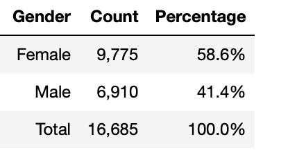
Note: The analysis completed in Table 2 and Fig 7 required additional cleansing to only include recorded split times. The total recorded usable entries for these analyses are as follows:

# create count column
gender2 = average_speed.groupby('Gender').size().reset_index(name='Count')

# create percentage column
gender2['Percentage'] = (gender2['Count'] / gender2['Count'].sum() * 100).round(1)

# add total row
total_row2 = gender2[['Count']].sum().rename({0: 'Total'})
total_row2['Percentage'] = (total_row2['Count'] / total_row2['Count'].sum() * 100).round(1)
gender2 = pd.concat([gender2, total_row2.to_frame().T])

# format percentage column elements
gender2['Percentage'] = gender2['Percentage'].astype(str) + '%'

# format Count column elements
gender2['Count'] = gender2['Count'].map('{:,.0f}'.format)
gender2 = gender2.reset_index()
gender2 = gender2.drop(columns=['index'])
gender2.loc[gender2.index[-1], 'Gender'] = 'Total'

# show 
gender2

Now it’s your time to run!

I hope you have enjoyed reading this article, and even better, I hope it has motivated you to run!

References

[1] https://results.sporthive.com/events/7037394564091167232

[2]https://www.runnersworld.com/uk/training/a774272/rules-of-running-runners-at-their-peak/#

Join thousands of data leaders on the AI newsletter. Join over 80,000 subscribers and keep up to date with the latest developments in AI. From research to projects and ideas. If you are building an AI startup, an AI-related product, or a service, we invite you to consider becoming a sponsor.

Published via Towards AI