Generalized Linear Mixed Models in SAS — distributions, link functions, scales, overdisperion, and…

Author(s): Dr. Marc Jacobs

Originally published on Towards AI the World’s Leading AI and Technology News and Media Company. If you are building an AI-related product or service, we invite you to consider becoming an AI sponsor. At Towards AI, we help scale AI and technology startups. Let us help you unleash your technology to the masses.

Statistics

Generalized Linear Mixed Models in SAS — distributions, link functions, scales, overdispersion, and normality of residuals.

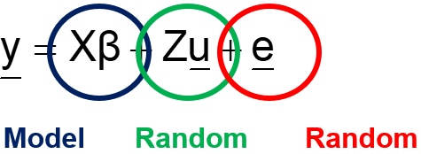
All statistical models have a systematic and a random part. In ANOVA and GLM models, the systematic part is the fixed effect and the random part is the error / unexplained variance. In mixed models, we have at least two random parts:

1. The variable intended to describe and use variance (e.g., block)
2. Error / unexplained variance

Our understanding of the world depends on the data that we collect and observe. This is why the design of our experiment is so important. Based on these observations, we build a statistical model which includes fixed and random parts. We build a model to describe/explain the world. We apply probability theory to the model to make inferences:

1. What is the chance that the model does not describe the world accurately?
2. What is the chance that what we have observed is due to chance? (which, of course, can never happen since chance by itself does not play a role)

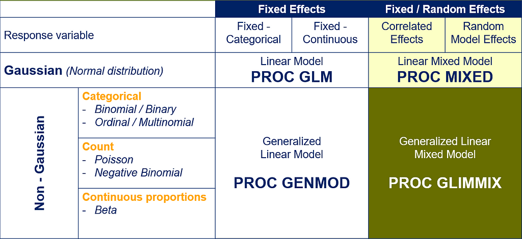
Linear Mixed Models (LMMs) can only analyze normally distributed data. In Generalized Linear Mixed Models (GLMMs), the response function (y) can come from different distributions. Whilst in LMMs we analyze the response directly, in GLMMs we need to apply a link function to transform the data IN the model

There are a lot of options available in SAS to do so.

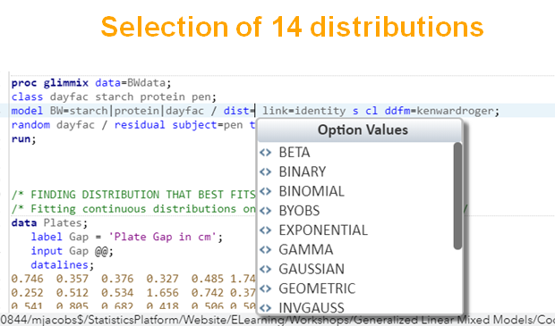
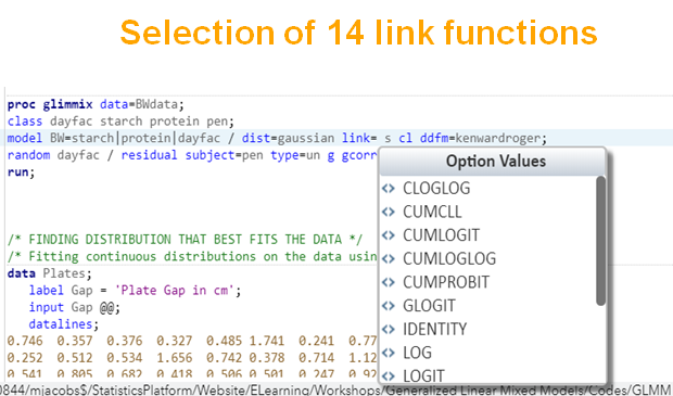
Below, is an example of data that needs to be log-transformed (either raw or inside the model) to be able to analyze it.

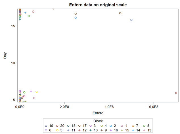
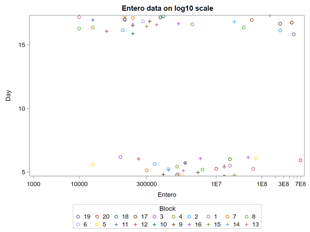
On data that comes from a log-normal distribution, using the normal distribution on the raw data is just plain wrong.

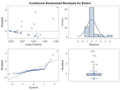
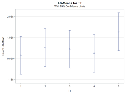
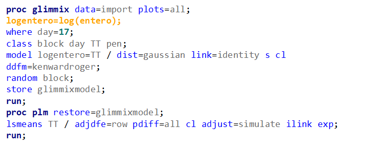
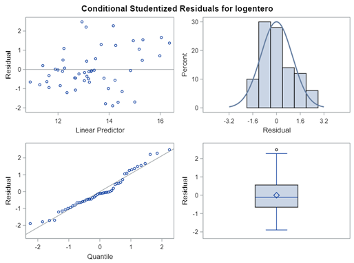
Now, let's use a different distribution instead. Since we transformed the data using a log transformation, we could opt for a lognormal distribution inside the model. This has the added benefit that an inverse transformation is done automatically.

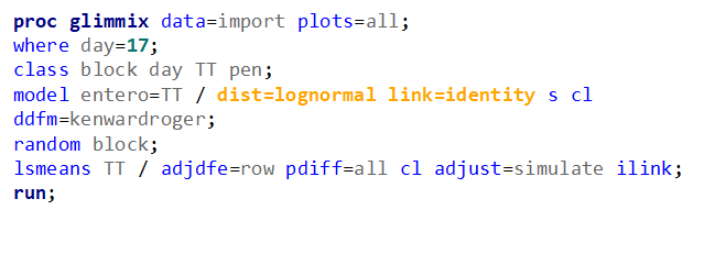
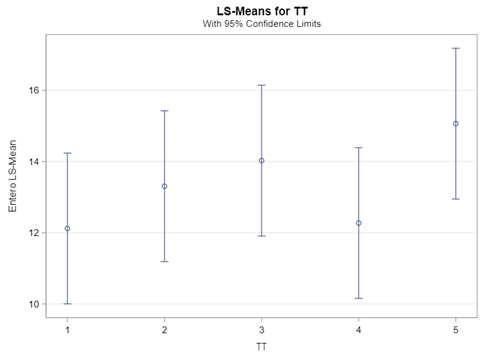
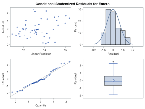
The data and model scale is the same in PROC MIXED since we only use the normal distribution. There is no link function in PROC MIXED. In PROC GLIMMIX, one determines the model scale by using the link function. The model scale will lead to non-observable estimates and non-linear functions of the response variable. They are used for inference. Then, one can revert to the data scale by using the ilink function in PROC GLIMMIX. The estimates are transformed to observables. This only works for means and not differences, since the link function is a non-linear function for which no closed formula back-transformation exists.

Link functions are typically nonlinear and so a difference is not preserved in a nonlinear function. Hence, applying the inverse link to a difference usually produces a nonsense result. To estimate differences on the data scale, you have to be smarter (for logit scales, you have odds ratios). The distribution and link can change when you estimate, the linear predictor never changes. Since we used the identity link (link=identity), the results were the same on the model scale and on the data scale. The identity link does not perform a transformation within the model

Lets use a new example in which we take observations coming from a binomial distribution.

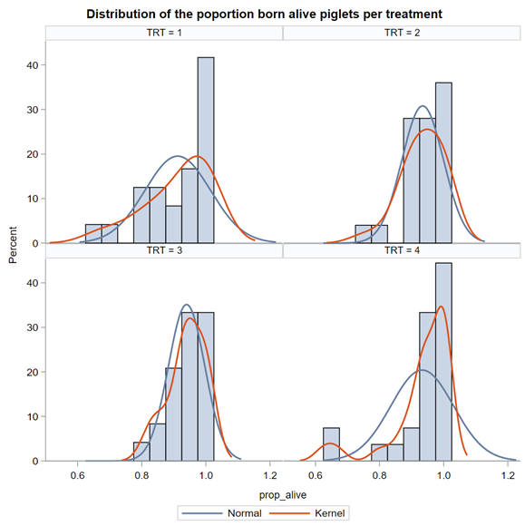
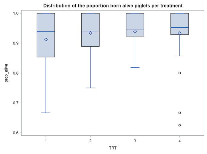
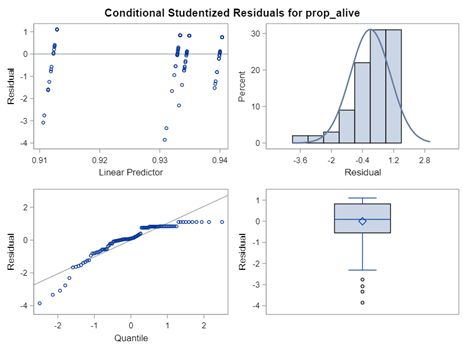
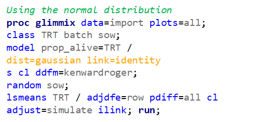
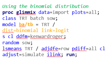
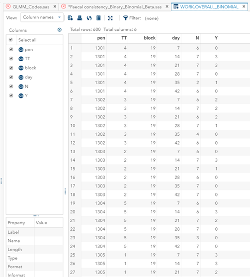
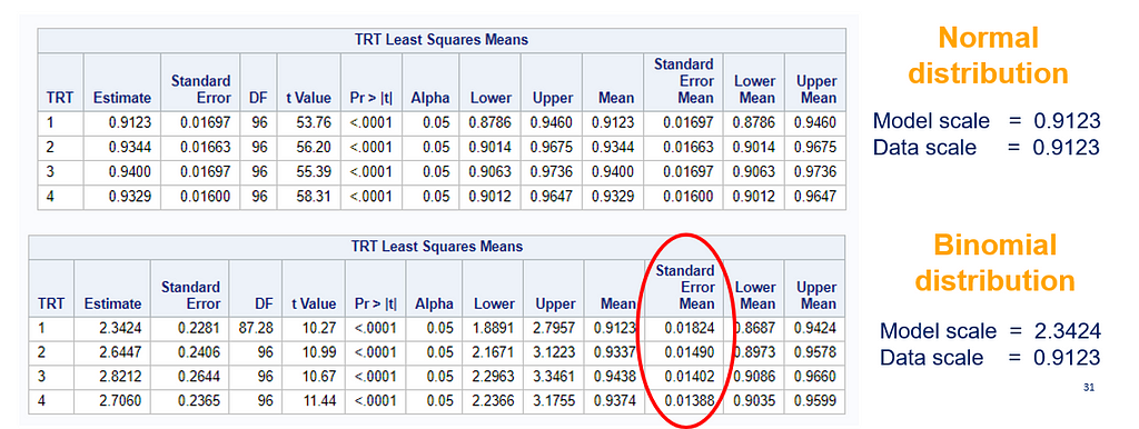
So, using the dist=binomial and link=logit instead of dist=Gaussian and link=identity has resulted in:

1. Smaller p-values.
2. Not being able to directly obtain the difference between two treatment proportions.
3. Having to resort to Odds Ratios to interpret treatment differences.

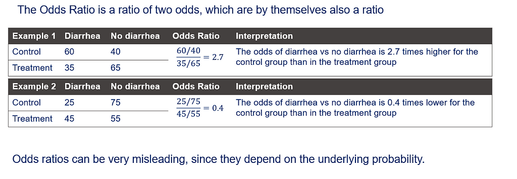
So, Linear Mixed Models (LMMs) can only analyze normally distributed data. Generalized Linear Mixed Models (GLMMs) can analyze all distributions. To do so, it needs to transform the data in the model using the link function (model scale). To obtain model results in the original scale (data scale) we use the inverse link. Using a GLMM for data with a non-normal distribution will provide you with the correct results! For Binomial Data, Odds Ratios will now have to be used to interpret treatment difference

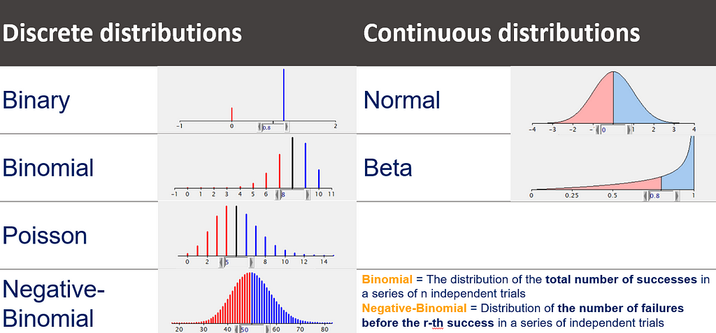
Lets talk more about probability and distributions. In statistics, a probability distribution is a mathematical function that provides the probabilities of occurrence of different possible outcomes in an experiment.

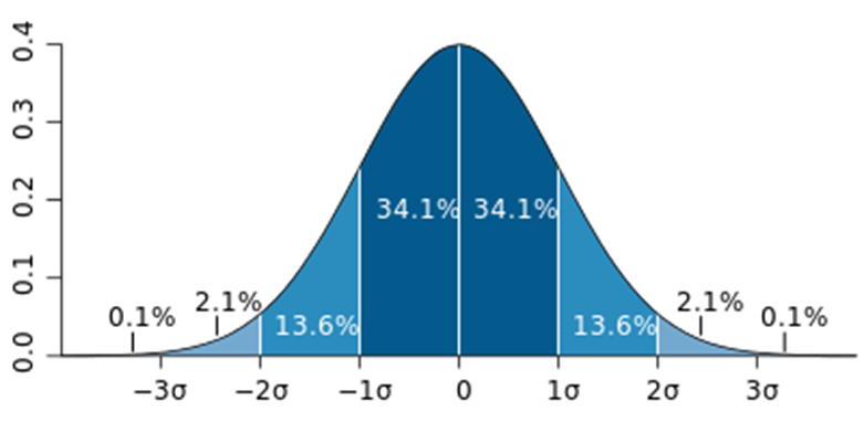
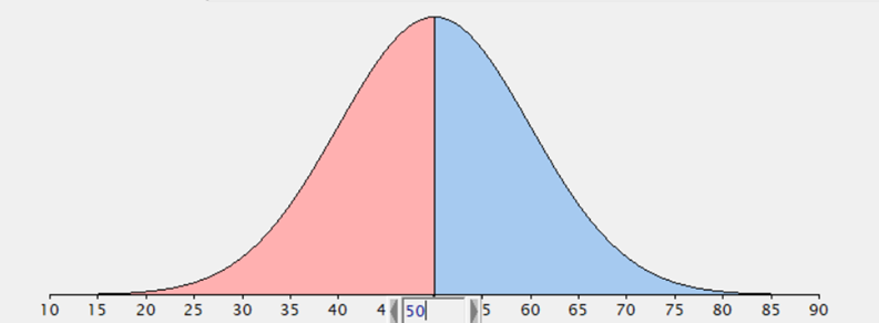
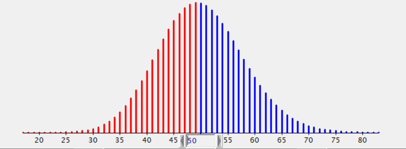
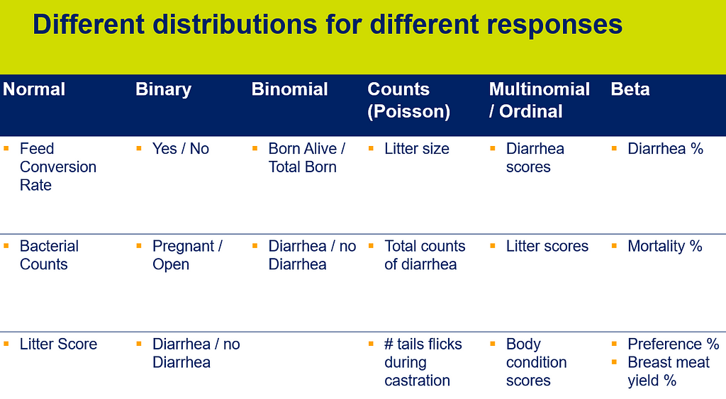
The probability distribution is different for continuous outcomes and discrete outcomes (integers). You can see some examples in the table below.

And if we are going to talk distributions, we absolutely NEED to talk about the mean-variance relationship which for the large part determines how distributions behave, and how useful they will be in analyzing different types of data.

The Normal Distribution is such a nice distribution because we can estimate the mean and the variance separately! Hence, if an underlying process is normal, it will be very easy to estimate the properties of the theoretical normal distribution!

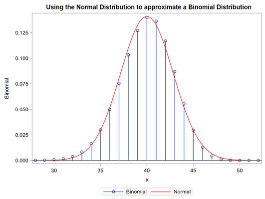
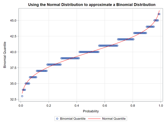
The difficulty of dealing with non-normal data is because there is a dependency between the mean estimator and the variance estimator. In addition, the data is discrete and thus no longer intuitive (many are taught about the normal distribution in high school). So, in the absence of a mean, we now have to talk about proportions and we use distributions to model the data as we see it, extrapolate it to the population, and base inference (p-values) on it. To do so, we have two major types of distributions — continuous and discrete.

The normal distribution is continuous, mostly used, and easiest to interpret since it has two parameters that can be estimated separately — mean & variance. For distributions in which the mean-variance relationship is linked, overdispersion occurs often — the variance is underestimated leading to false positives.

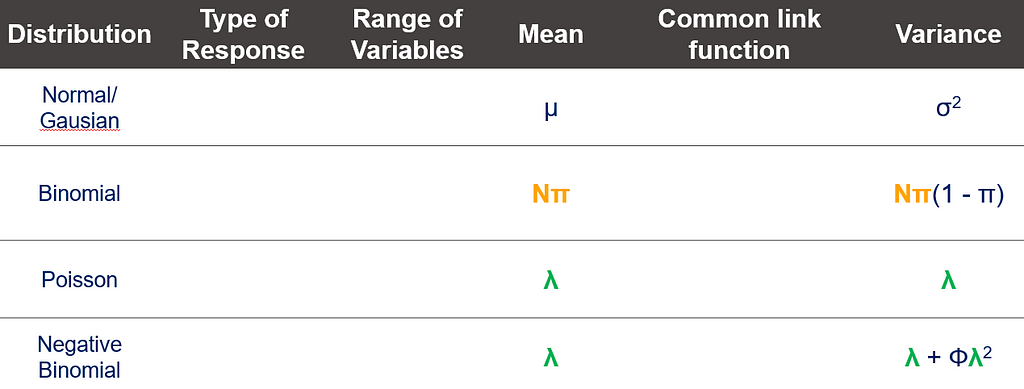
And so we arrive at the topic of overdispersion, which is where the mean-variance relationship becomes extremely interesting. Below, you see the characteristics of four distributions and how their mean and variance are specified. The Poisson Distribution immediately sticks out.

Overdispersion was briefly mentioned in the previous part and is something we will highlight further before proceeding to the more practical examples. Overdispersion is not an issue in Linear Mixed Models as LMMs only deal with data coming from a Normal Distribution, and in a Normal Distribution, the variance is estimated separately from the mean. In GLMMs, however, some form of dispersion is practically always present, meaning that the variance is either underestimated (overdispersion) or overestimated (underdispersion).

Let's use an example to make the issue clear.

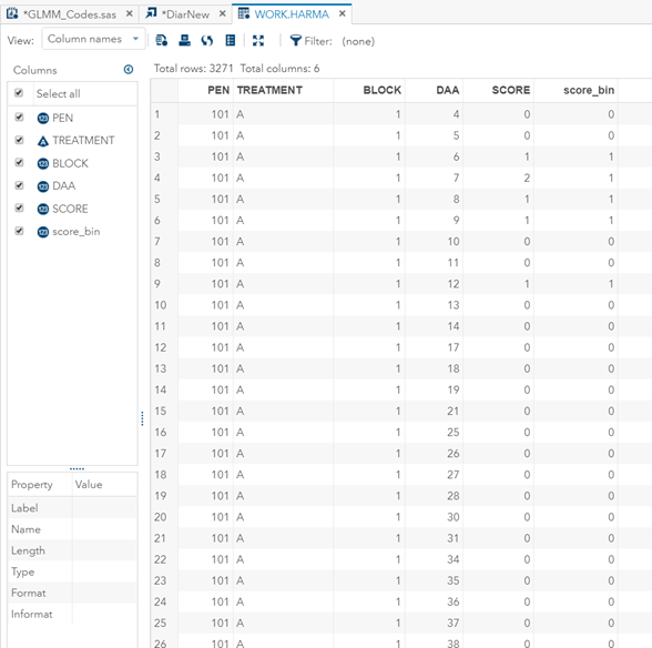
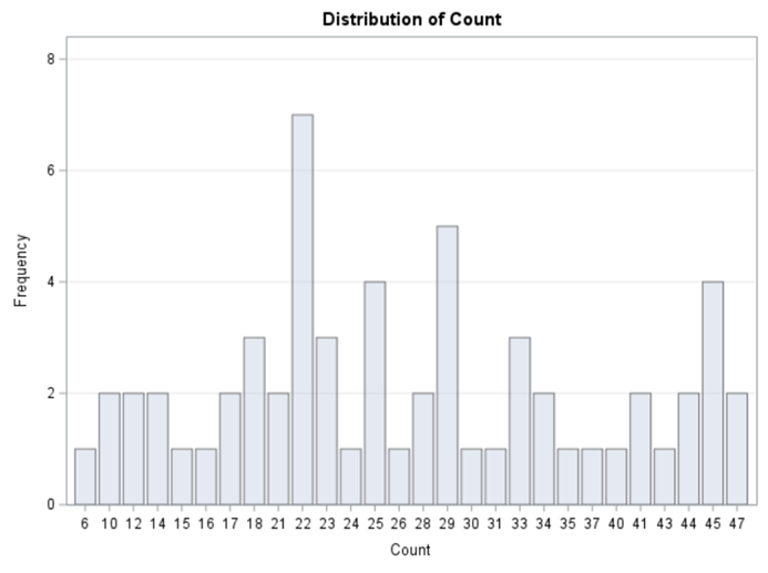
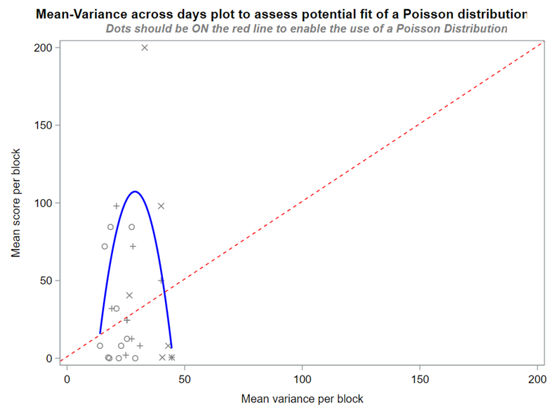
A simple and straightforward way to assess if the Poisson is a good distribution to fit is to plot the mean-variance relationship across groups. The dots should be on the red line.

Overdispersion often happens because the linear predictor is not complete which is a result of not having included enough / the most important variables. To detect overdispersion, you need to look if there is more variance in the model than expected, given the sample size, by dividing the variance detected by the degrees of freedom. To get this metric you need to change the estimation method in GLIMMIX, which opens quite some complex statistical theories:

1. Pseudo-Likelihood
2. Laplace (method=laplace)
3. Quadrature (method=quad(qpoints=5))

Option two or three cannot be used in PROC GLIMMIX if you have a random/residual statement included. To check numerically for overdispersion, you can take a look by dividing the Pearson Chi-Square divided by the Degrees of Freedom. If the value is between 0.5–1.5 you are OK, but there is no official cut-off.

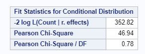
In this example, we actually detect underdispersion. When there is no dispersion, the Pearson Chi-square / DF value should be 1 — meaning that the variance is estimated correctly based on the degrees of freedom present. A value outside of the range [ 0.5; 1.5 ] would constitute too much dispersion. In extreme cases, you will see a value between 5 and 10, meaning that we underestimate the variance by a factor of 5 or 10

Let's test all of this using an example:

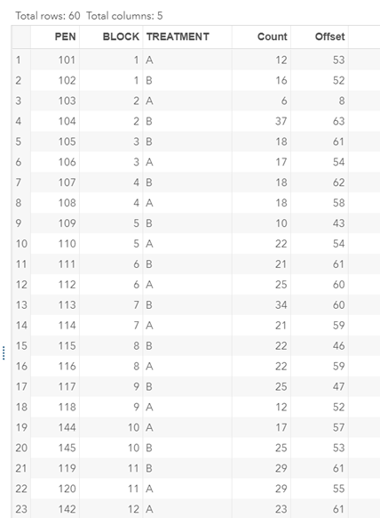
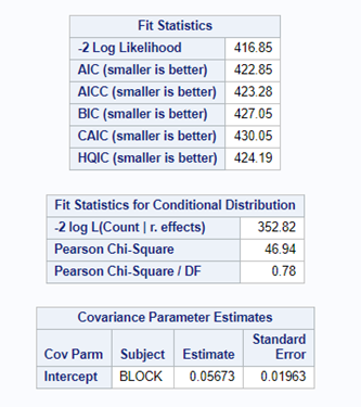
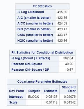
To recap, in the Normal Distribution, the mean and variance are estimated separately. In other distributions, the variance (e.g., Poisson, Binomial, Beta) is a function of the mean. This often creates overdispersion — an underestimate of the variance leading to false positives. Underdispersion is less common but can surely happen. In both cases, the best approach is changing the distribution towards one that provides you with more freedom to model.

In most models, there is the assumption that the residuals from a model are i.i.d — independent and identically distributed random variables. How this works, you can see from a simulation down below.

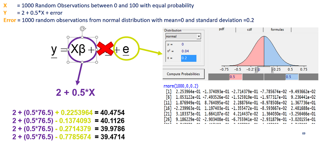
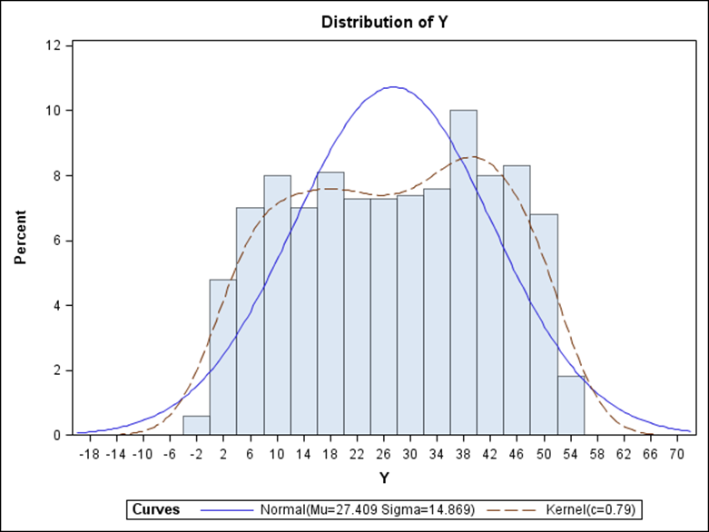
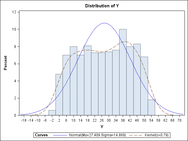
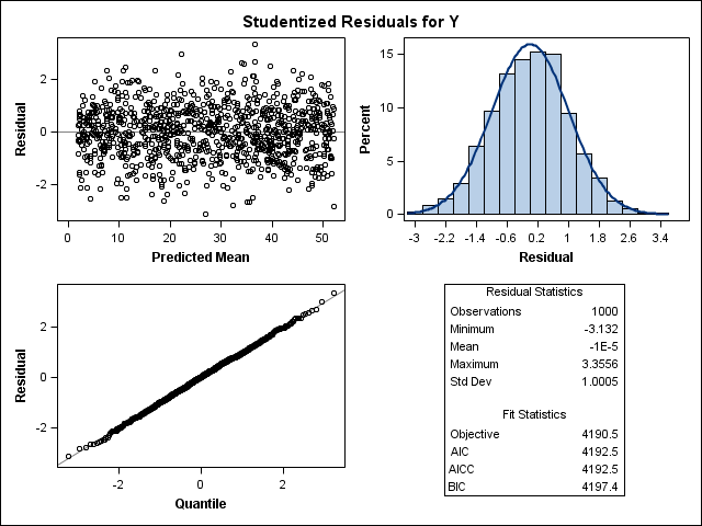
Now, let's simulate a Poisson distribution and see what the residuals will look like.

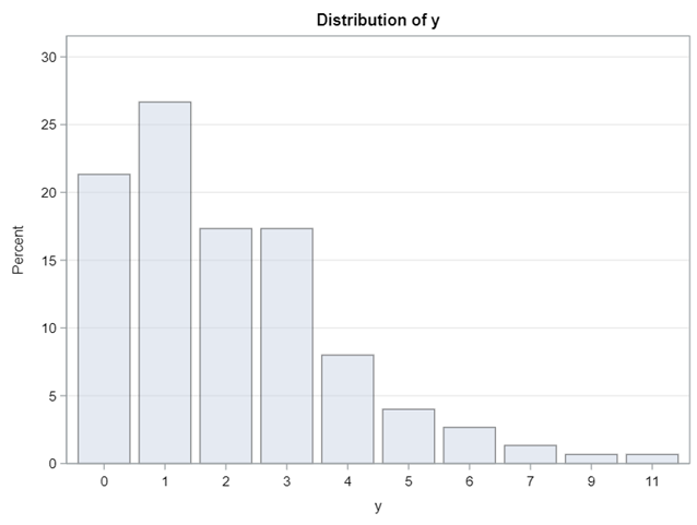
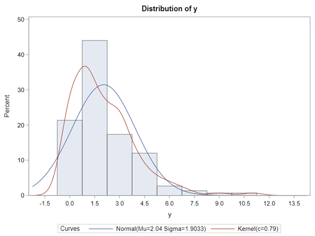
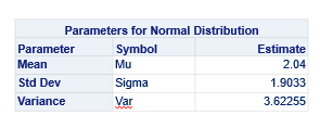
The Poisson distribution based on the mean looks different than a distribution based on the variance. In a Poisson distribution, a larger λ will cause a longer tail. Let's see what happens if we start modeling the data.

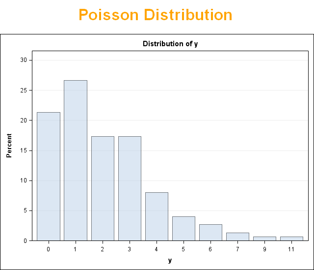
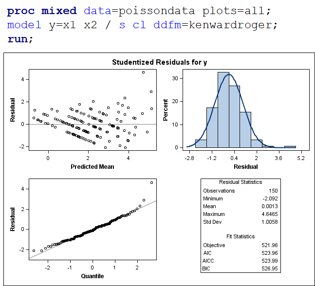
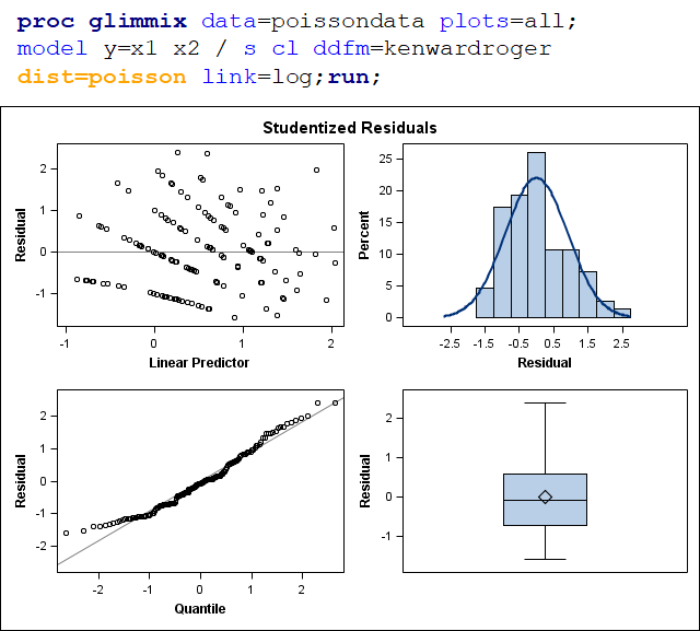
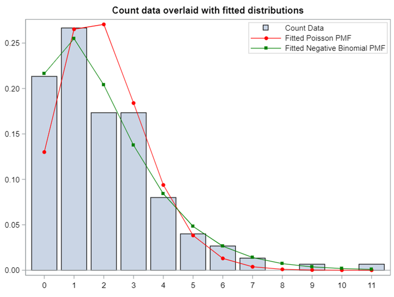
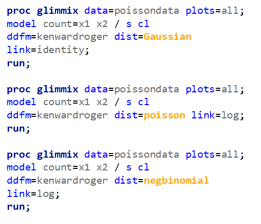
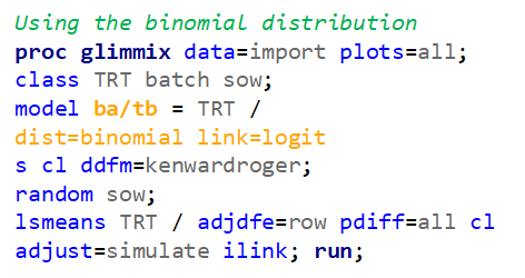
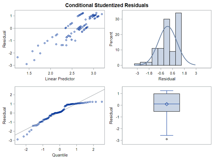
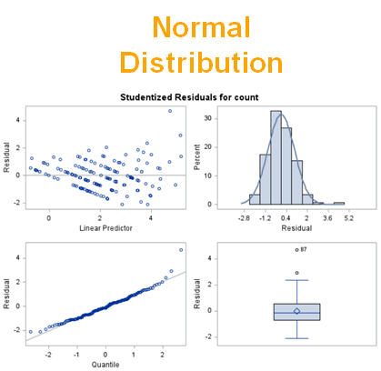
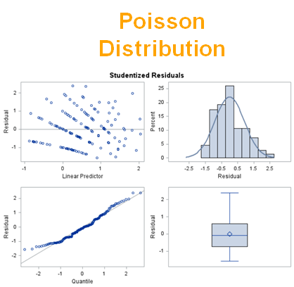
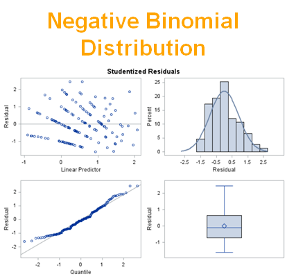
The above exercise has valuable lessons:

1. Do NOT use the plots from the GLIMMIX model to assess if one model is better than the other.
2. Stick to the Information Criteria described in the Linear Mixed Model course.
3. It is best to look at the LSMEANS, the standard errors, and metrics for over/underdispersion
4. In Generalized Linear Mixed Models, the errors cannot come from a normal distribution

Hence, using the residual plots to assess model fit and comparing models is tricky and will lead to incorrect results, even if they look as you are used to. It is best to look at the LSMEANS, the standard errors, and metrics for over/underdispersion.

Hope you enjoyed this! More to come on specific types of data and how to deal with them!

---

Generalized Linear Mixed Models in SAS — distributions, link functions, scales, overdisperion, and… was originally published in Towards AI on Medium, where people are continuing the conversation by highlighting and responding to this story.

Join thousands of data leaders on the AI newsletter. It’s free, we don’t spam, and we never share your email address. Keep up to date with the latest work in AI. From research to projects and ideas. If you are building an AI startup, an AI-related product, or a service, we invite you to consider becoming a sponsor.

Published via Towards AI