Elucidating the power of Inferential Statistics to make smarter decisions!

Author(s): Harjot Kaur

Originally published on Towards AI the World’s Leading AI and Technology News and Media Company. If you are building an AI-related product or service, we invite you to consider becoming an AI sponsor. At Towards AI, we help scale AI and technology startups. Let us help you unleash your technology to the masses.

Elucidating the Power of Inferential Statistics To Make Smarter Decisions!

The lost importance of inferential statistics…

The strategic role of data science teams in the industry is fundamentally to help businesses to make smarter decisions. This includes decisions on minuscule scales (such as optimizing marketing spending) as well as singular, monumental decisions made by businesses (such as how to position a new entrant within a competitive market). In both regimes, the potential impact of data science is only realized when both humans and machine actors are learning from the data and when data scientists communicate effectively to decision-makers throughout the business. There certainly exists a duality between inference and prediction throughout the machine learning lifecycle. From a balanced perspective, prediction and inference are integral components of the process by which models are compared to data.

However, an imbalanced, prediction-oriented perspective prevails in the industry where data scientists tend to jump straight into predicting the target variable. This approach may prove detrimental to making smarter decisions.

Through this blog, I offer to explain the true power of inference and prediction, working for hand in glove.

The Duality of Prediction and Inference

Typically a simple supervised machine learning setup begins with data — composed of independent and dependent variables. Both variables have an underlying existential relationship, which is often given as Y = f(β.x)

This setup is explained through a graphical diagram given below:

Now, let’s attempt to decompose the above diagram into prediction and inference. Before that, for all practical purposes, let me define both terms in the most simplistic way possible.

• Predictions: The outputs emitted by a model of a data generating process in response to a specific configuration of inputs.
• Inferences: The information learned about the data generating process through the systematic comparison of predictions from the model to observed data from the data generating process.

A supervised machine learning setup with a balanced perspective, valuing both predictive and inference components can be put down as:

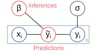
The above figure illustrates that prediction and inference are two distinct goals of the modeling process, which both offer value to organizations and are inextricably connected in the modeling process, but can be viewed in different ways. Both perspectives are valid in different contexts, and analysts and organizations need to consider and recognize the appropriate orientation for a particular data science project.

Let’s test the power of inferential statistics!

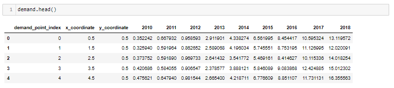
Here, let me explain the duality of inference and prediction with an example. Let’s assume we aim to predict the demand for EV scooters in 2019 for a certain region, and we have been provided with historical yearly demand for EV scooters for the same region. Given the setup, let’s deliberate on the equal value generation from both inference and prediction components.

Reading the data — below data indicates for every demand point index, we have been given historical demand for EV scooters. Here, demand for EV scooters in 2018 becomes the dependent variable(Y), and historical demand values are the independent variables(x)

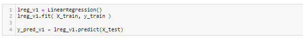
Demand prediction using Linear Regression- We can quickly predict demand for EV scooters using linear regression and evaluate the model errors using RMSE.

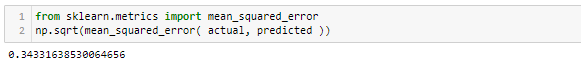
Here, an RMSE of 0.34 is exceptional. So, I should look no further and quickly get done with the predictions for the subsequent years.

But wait! What do we know about the parameters or significant variables or explainability of the model or perhaps which model performs better and why?

This learning comes from the inference component of the supervised machine learning setup and should be considered as vital as the prediction component.

Let’s attempt to answer a few questions here using the regression summary table.

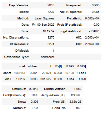
Firstly, let me break this summary table into 3 sections.

(1) The first section lists measures that explain the regression model fitment, i.e., how well the regression model can “fit” the dataset. The following measures help us understand the overall model fitment.

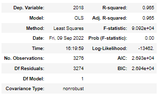
• R-squared — this is often written as r2 and is also known as the coefficient of determination. It is the proportion of the variance in the response variable that can be explained by the predictor variable. The value for R-squared can range from 0 to 1. A value of 1 indicates that the response variable can be perfectly explained without error by the predictor variable. In this example, the R-squared is 0.965, which indicates that 96.5% of the variance in demand for EV scooters can be explained by the historical demand figures.
• F-statistic- This statistic indicates whether the regression model provides a better fit to the data than a model that contains no independent variables. In essence, it tests if the regression model as a whole is useful. Generally, if none of the predictor variables in the model are statistically significant, the overall F statistic is also not statistically significant. This statistic can be largely useful to test amongst many models with different independent variables which model fits better.

Likewise, AIC and BIC also help gain a similar insight about the model fitment.

(2) The second section helps translate inferences around the coefficient estimates, the standard error of the estimates, the t-stat, p-values, and confidence intervals for each term in the regression model.

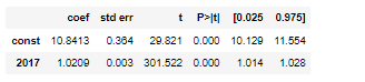
• Coefficients — The coefficients give us the numbers necessary to write the estimated regression equation. In this example, the estimated regression equation is:

Demand for EV scooters in 2019 = 10.84 + 1.02 * Demand for EV scooters in 2017

Each coefficient is interpreted as the average increase in the response variable for each one unit increase in a given predictor variable, assuming that all other predictor variables are held constant. For example, for each unit of EV scooter sold in 2017, the average expected increase in demand in the subsequent year is 1.02 units, assuming everything else is held constant. The intercept is interpreted as the expected average units of demand for EV scooters without considering their historical demand.

• Standard error and p-value — The standard error is a measure of the uncertainty around the estimate of the coefficient for each variable. The p-value number tells us if a given response variable is significant in the model. In this example, we see that the p-value for demand in 2017 is 0.000. This indicates that demand in 2017 is a significant predictor of demand in 2018.
• Confidence Intervals for Coefficient estimates- The last two columns in the table provide the lower and upper bounds for a 95% confidence interval for the coefficient estimates. For example, the coefficient estimate for demand in 2017 is 1.02, but there is some uncertainty around this estimate. We can never know for sure if this is the exact coefficient. Thus, a 95% confidence interval gives us a range of likely values for the true coefficient. In this case, the 95% confidence interval for demand in 2017 is (1.014, 1.028).

(3) The last section provides us with an inference about the residuals or errors. Let’s look at each of the values listed:

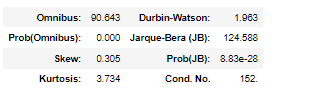
• Omnibus/Prob(Omnibus) — a test of the skewness and kurtosis of the residual. We hope to see a value close to zero, which would indicate normalcy. The Prob (Omnibus) performs a statistical test indicating the probability that the residuals are normally distributed. We hope to see something close to 1 here. In this case, Omnibus is relatively high, and the Prob (Omnibus) is low, so the data is not normal.
• Skew — a measure of data symmetry. We want to see something close to zero, indicating the residual distribution is normal. Note that this value also drives the Omnibus.
• Kurtosis — a measure of “peakiness”, or curvature of the data. Higher peaks lead to greater Kurtosis. Greater Kurtosis can be interpreted as a tighter clustering of residuals around zero, implying a better model with few outliers.
• Durbin-Watson — tests for homoscedasticity. We hope to have a value between 1 and 2. In this case, the data is close but within limits.
• Jarque-Bera (JB)/Prob(JB) — is like the Omnibus test in that it tests both skew and kurtosis. We hope to see in this test confirmation of the Omnibus test.
• Condition Number — This test measures the sensitivity of a function’s output as compared to its input. When we have multicollinearity, we can expect much higher fluctuations to small changes in the data. Hence, we hope to see a relatively small number, something below 30. In this case, we are way over the roof at 152.

So, to summarize, in this case, the regression summary table has far more things to say than the RMSE from the prediction component. We have got answers to pivotal questions such as (a) model fitment, (b) insight into significant variables and their attached standard error, and a deep dive into residuals.

Visibility and correct interpretation of parameters provide us with better control to make smarter decisions.

In a nutshell, a balanced perspective on both prediction and inference is pivotal to making smart decisions. Both components must function hand in glove to make the machine learning model meaningful and useful for businesses.

Lastly, thank you for your patience in reading up till the end and if you’ve found this write-up useful, then give me a clap or two! and if not, do write back with your comments and questions; I will be happy to answer and connect for a discussion on Linkedin.

References:

• https://hdsr.mitpress.mit.edu/pub/a7gxkn0a/release/7
• https://www.statology.org/read-interpret-regression-table/
• https://medium.com/swlh/interpreting-linear-regression-through-statsmodels-summary-4796d359035a
• https://www.accelebrate.com/blog/interpreting-results-from-linear-regression-is-the-data-appropriate

Elucidating the power of Inferential Statistics to make smarter decisions! was originally published in Towards AI on Medium, where people are continuing the conversation by highlighting and responding to this story.

Join thousands of data leaders on the AI newsletter. It’s free, we don’t spam, and we never share your email address. Keep up to date with the latest work in AI. From research to projects and ideas. If you are building an AI startup, an AI-related product, or a service, we invite you to consider becoming a sponsor.

Published via Towards AI