Dynamic Time Warping on Time Series Analysis

Author(s): Sumeet Lalla

Originally published on Towards AI the World’s Leading AI and Technology News and Media Company. If you are building an AI-related product or service, we invite you to consider becoming an AI sponsor. At Towards AI, we help scale AI and technology startups. Let us help you unleash your technology to the masses.

Introduction

Agriculture plays a very important role in a developing country like India. It contributed about 20 percent to the GDP, and 58 percent of the Indian population is linked to Agriculture. Wheat is one of the staple foods in India. Machine Learning plays a big role in Agriculture in the various stages of harvesting to improve crop yield, forecasting of weather, identification of diseases and pests, etc.

The seasonal growth of wheat is studied for the months from October 2020 to May 2020 for the three districts in India, i.e., Karnal, Kaithal, and Dewas. The metric used to study the same is Vegetation Index which is normalized (termed NDVI) and precomputed from Sentinel-2 satellite data. The training data comprises the geographical information of the district, i.e., latitude and longitude, along with the information if wheat can be produced on it or not. It also contains the NDVI data from the date of germination till harvest for each sector in the district, which is the primary key for the former and acts as a foreign key for the latter.

The given problem involves the NDVI time series for the seasonal growth of wheat in three districts of India. The data for each district constitutes the NDVI time series which can have different starting and ending dates, i.e., the start of germination and end of harvest. Hence the length of the time series is sometimes varying. We came up with an approach to compare two-time series using Dynamic Time Warping.

The NDVI time series for the districts is analyzed for similarity using Dynamic Time Warping (DTW). The DTW is used as feature embeddings and as a metric for 1NN classification. The two approaches are applied to the test data, and evaluation metrics are compared. For the feature embeddings, two classifiers, i.e., Support Vector Machine and tree-based ensemble methods, are used. In the case of the tree-based ensemble method, Random Forest Classifier was used. The evaluation results of the two classifiers are checked for the individual as well as combined districts, and the scenarios are analyzed and discussed for cases where one classifier outperforms the other.

Motivation Of Work

The similarity between the time series using Dynamic Time Warping as feature embeddings as well as metric for 1NN classification have been analyzed before on UCR datasets as well as on temporal sequences in audio and speech synthesis and signal analysis domain and is used extensively for time series classification.

We have analyzed Dynamic Time Warping as feature embeddings for out-of-phase time series data which is collected from Landsat and Sentinel 2 satellites. These have been analyzed by using Dynamic Time Warping as a metric for 1NN classification and as feature embeddings, and a comparison of the effectiveness between the two has been made.

Structure Of Work

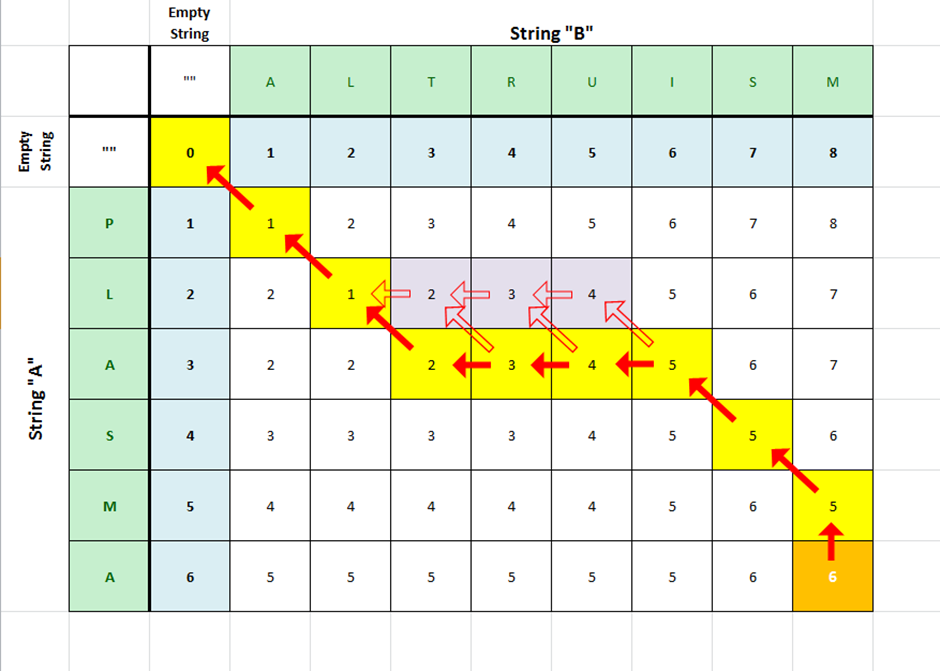
DTW follows the edit distance algorithm where the time series are treated as subsequences and warping is calculated among all possible points of the time series. It basically signifies the alignment distance between the time series, and its value denotes the alignments needed to convert the compared time series to the reference one. The detailed algorithm for Dynamic computing Time Warping, along with its properties, is detailed in the next sections.

The Dynamic Time Warping distance finds its usage in audio signal analysis, satellite image analysis, etc. It, however, cannot be a norm as the properties of the norm are violated, which will be discussed in the next sections.

Related Work

Some of the noticeable work in this field which was referred to as part of this project, are as under:

Dynamic time warping with out-of-phase time series is analyzed in the paper (Maus et al., 2016), where time series of varying lengths are handled by introducing the Time-Weighted Dynamic Time Warping Method. Here Dynamic Time Warping is used as a metric.

Dynamic Time Warping as feature embeddings is analyzed in the paper (Kate, 2015). Here the author proposes to use Dynamic Time Warping as a feature.

The paper (Young-Seon, Jeong, & Omitaomu, 2011) discusses the out-of-phase time series and the different penalizing functions that can be applied to the same for constraining the Dynamic Time Warping between them.

Dynamic Time Warping:

Given two-time series X=x1, x2, x3…, xn and Y=y1, y2, y3…, ym, the simplest distance metric which can be computed between the two is Euclidean Distance provided m=n.

The Euclidean distance metric is quite simple to use and effective hence it is widely used in data mining tasks. However, the simplicity comes with a disadvantage in Time Series tasks as the Euclidean distance metric penalizes more for a small variation in distance between the Time Series due to the square term. The small variation can be due to the Time Series starting slightly earlier/later or completing earlier/later. The other disadvantage is that the Time Series needs to have an equal length to compute it. Both the above-discussed disadvantages in Time Series can be overcome by using Dynamic Time Warping.

Dynamic Time Warping tries to find the best alignment between the time series, X=x1, x2, x3…, xn and Y=y1, y2, y3…, ym. To align the time series, the concept of edit distance algorithm using dynamic programming is used. The alignment which is the best will minimize the overall cost between the points on the time series. The cost, in this case, is the norm, either 1-norm, also called Manhattan distance, or 2-norm, also called Euclidean Distance. Generally, it is denoted by p norm.

The algorithm is described below.

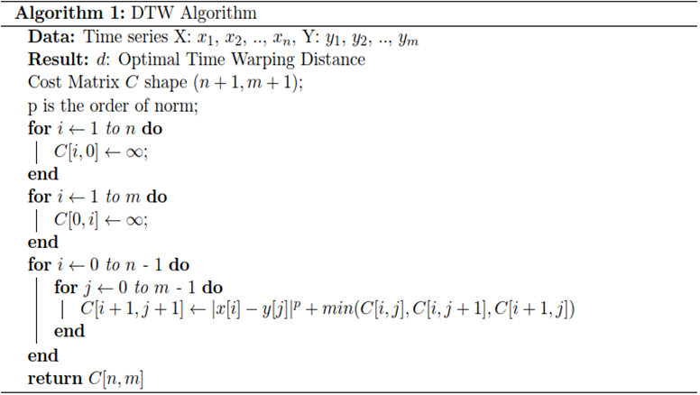
The overall computational complexity of computing Dynamic Time Warping is O(mn), where m and n are the lengths of the time series. From the above, it can be concluded that it is a computationally expensive process. Various speedups have been introduced, like introducing a lower bound to the distance or introducing a window of size r, which restricts the warping path to be closer to the diagonal of the cost matrix. This helps to improve the computational speed of calculating Dynamic Time Warping as well as improving the accuracy of time series classification.
In our case, the constraint we would be using is time-weighted, which is a penalty cost function depending on the date of the time series, and penalizing the Dynamic Time Warping on the same, which will be discussed in the next sections.

Properties of Dynamic Time Warping

a) The Dynamic Time Warping is symmetric if the step pattern chosen is symmetric while computing the alignment from test to reference point else, it is asymmetric.

b) The Dynamic Time Warping between two similar sequences is 0.

c) The Dynamic Time Warping does not follow triangular inequality.

The third property c) above tells us that Dynamic Time Warping violates the norm properties and hence cannot be treated as a norm and hence as a Metric. Thus, it can be treated as a Measure. The first two properties of Dynamic Time Warping will be used when computing the Dynamic Time Warping matrix between the reference and test point discussed in the next sections.

Optimal Path for Dynamic Time Warping (DTW)

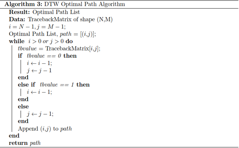
In the above-discussed DTW algorithm, to trace back the optimal path, a traceback matrix is maintained, which stores the decision, i.e., matching, insertion, and deletion made when computing the Dynamic Time Warping during intermediate steps of Dynamic programming. A path list is used, which is initialized with the end indices of the time series, X and Y. The path list is then appended with the other indices of the time series, X and Y, based on the traceback matrix. The indices are incremented/decremented based on the value of the traceback matrix at the given indices iteratively. The length of the optimal path is simply the count of the number of elements in the path list.

The algorithm is described below.

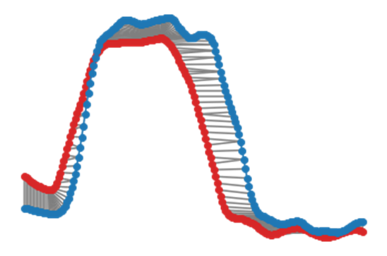
Time Series Plot (from Example dataset)

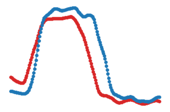
Naïve DTW Cost Matrix and Time Series Alignment (from Example dataset)

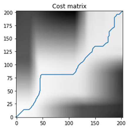
From the above plot of the cost matrix, we can observe that there are incorrect alignments leading to the optimal path being away from the diagonal. We will observe in the next chapter how the Time Weighted Dynamic Time Warping reduces the incorrect alignments by penalizing the incorrect warpings leading to the optimal path being closer to the diagonal.

From the above plot, we observe that the Naïve DTW produces incorrect alignments, which would be corrected when we use the Time Weighted Dynamic Time Warping described in the next chapter.

Time Weighted Dynamic Time Warping:

The previous chapter discussed the original implementation of Dynamic Time Warping. From it, we can conclude that it applies equal weight while computing the distance between the test and reference point. However, there can be a scenario where there are phase differences between the test and reference point. The original implementation does not handle it. In the paper (Young-Seon, Jeong, & Omitaomu, 2011), the weight cost function is proposed to overcome the problem of phase differences between the test and reference point. The points in the sequence are prevented from matching further to the other sequence by using a penalty which in turn reduces the rate of misclassification. Our problem is related to the NDVI time series, and NDVI is calculated using the pixel of the image for the date. Hence, this problem falls under the space-time classification category. As proposed in the paper (Maus et al., 2016), we would be proceeding with the modified weighted logistic cost function, which has midpoint β and steepness α.

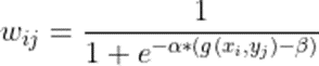
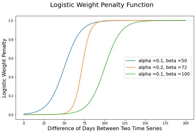
Let us walk through the above equation of computing the penalty for the time series X and Y described above. The wij denotes the penalty and the α and β are hyperparameters that represent the steepness and the midpoint of the logistic function and can be obtained by running different experiments on the train and test data. The g(xi, yj) is a function denoting the day’s difference between the dates of xi and yj of two-time series X and Y described above. The below plot shows the value of penalty wij for different values of hyperparameters, i.e., α and β.

The penalty function value computed from above is added to the Dynamic Time Warping distance computation algorithm described below.

Time Weighted DTW Cost Matrix and Time Series Alignment (from Example dataset) with α=0.001 and β=20

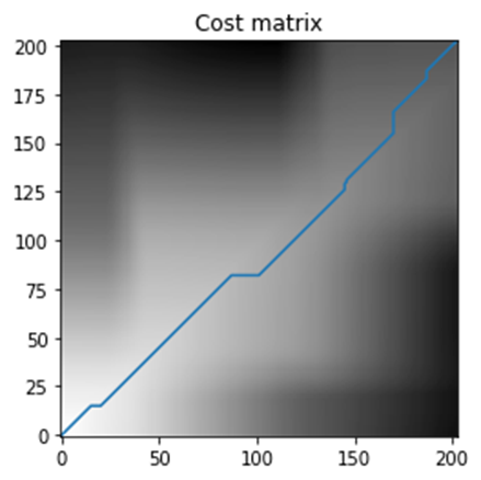
From the above plot, we observe that the Time Weighted Dynamic Time Warping reduces the incorrect alignments by penalizing the incorrect warpings leading to the optimal path being closer to the diagonal.

From the above plot, we observe that the Time Weighted Dynamic Time Warping reduces the incorrect alignments by penalizing the incorrect warpings when compared with Naïve DTW.

Conclusion

The Classifier Model developed as part of this project is able to predict the growth of wheat in different districts individually as well as combined. Further, the study yielded the following important observations:

a) The Time Weighted DTW individual model on each of the districts performs better than the merged model.

b) Using Time Weighted DTW as feature embeddings for classification gives better evaluation results on test data than when using it as a metric for 1NN classification.

c) When using Time Weighted DTW as feature embeddings, use SVC as the classifier since it handles the problem of the number of predictors, i.e., the number of features >> number of observations in the dataset.

References

1. Kate, J. R. (2015). Using Dynamic Time Warping Distances as Features. Springer, 28.

2. Maus, V., Camara, G., Cartaxo, R., Sanchez, A., Ramos, M. F., & Ribeiro, Q. G. (2016). A Time-Weighted Dynamic Time Warping method for land use and land cover mapping. IEEE JOURNAL OF SELECTED TOPICS IN APPLIED EARTH OBSERVATIONS AND REMOTE SENSING, 10.

3. Young-Seon, J., Jeong, K. M., & Omitaomu, A. O. (2011). Weighted dynamic time warping for time series classification. Elsevier, 10.

---

Dynamic Time Warping on Time Series Analysis was originally published in Towards AI on Medium, where people are continuing the conversation by highlighting and responding to this story.

Join thousands of data leaders on the AI newsletter. It’s free, we don’t spam, and we never share your email address. Keep up to date with the latest work in AI. From research to projects and ideas. If you are building an AI startup, an AI-related product, or a service, we invite you to consider becoming a sponsor.

Published via Towards AI