Dataset Used:-

Author(s): Pushkara Sharma

Originally published on Towards AI.

Natural Language Processing, Programming

Automatic Moderator for StackOverflow Questions

In this article, we will try to build a machine learning model that will automatically predict the quality of the question asked by the person and assign it with the tag accordingly.

If you are new to Machine Learning, It's OK. I will try to elaborate on every step in beginner’s friendly language. It is a great project to showcase your skills and as I have used libraries for most of the tasks, it will be easy for you to explain the work to others.

Since questions consist of language(words/sentences), it is a Natural Language Processing(NLP) problem. NLP is just a part of A.I. that deals with human language(speech/text). Google translator is one of the best examples of NLP.

Now, as we are clear about NLP and our problem statement, Let's directly jump to the coding sectionU+1F60E.

I have used the dataset “60k Stack Overflow Questions with Quality Rating” that is available on Kaggle. There are three categories for quality:-

• LQ_CLOSE = Low-quality posts that were closed by the community
• LQ_EDIT = Low-quality posts that remain open after some changes.
• HQ = High-quality posts with a total of 30+ score

But the dataset there is split into training and testing. If you want a single CSV file you can get it in my GitHub repo.

Prerequisites:-

I assume that you are familiar with python and already have installed python 3 in your systems. I have used a jupyter notebook for this tutorial. You can use the IDE of your like.

Installing Required Libraries

For this project, you need to have the following packages installed in your python. If they are not installed, you can simply usepip install PackageName . Although most of these libraries come inbuilt in anaconda suite.

• pandas — for data analysis and performing manipulation on data
• matplotlib — for creating basic plots
• seaborn — used for creating more attractive plots
• re(Regular Expression) — for checking the matched string
• nltk — for performing natural language processing tasks.
• sklearn — for splitting and vectorizing data(that’s what we have used for)
• xgboost — ensemble machine learning algorithm

Let’s Start Coding!

Here, firstly we have to import all the libraries that we will use. Pandas will be used to manipulate our dataset. Matplotlib will help us to create simple plots like bar charts. Seaborn will create some advanced good looking plots. re(regular expression) is used for removing unwanted text from the questions. nltk(Natural Language Toolkit) here is used only to get stopwords(words like is,the,of that do not contribute to our model). The last line here is used to download the stopwords.

import pandas as pd
import matplotlib.pyplot as plt
import seaborn as sns
import re
import nltk
nltk.download('stopwords')

Now, we have simply created the dataframe df by loading our dataset. And as a good practice, we have printed the shape of the dataframe that comes out to be (60000,7). Then we have printed the first 5 rows of the dataframe.

df = pd.read_csv("data.csv")
print(df.shape)df.head()

There are 7 columns in the dataframe, but we are only interested in title, body, and y(label). So, we have simply dropped the columns that are not required for our classification task.

df = df.drop(['Id','Tags','CreationDate','Unnamed: 0'],axis=1)
df.head()

Now, we would like to perform some exploratory analysis of our data. So, we have extracted the number of words in Title, Body, and also the total words combined of both. Then we have printed our dataframe as you can see from the screenshot below.

#Number Of words in Selected Text
df['Num_words_body'] = df['Body'].apply(lambda x:len(str(x).split()))
#Number Of words in main text
df['Num_words_title'] = df['Title'].apply(lambda x:len(str(x).split())) 
#Total Number of words text and Selected Text
df['Total_words'] = abs(df['Num_words_body'] + df['Num_words_title'])df.head()

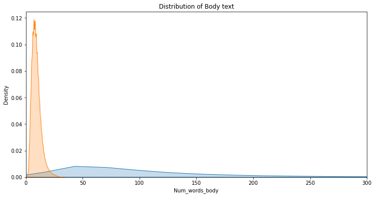
Visualization is very important in analysis. Here, firstly we define the size of our figure. Then we define the KDE plot(Kernel Density Estimation) for Num_words_bodyand Num_words_title . Kdeplot is used for visualizing the probability density of continuous variables. Finally plt.xlim is used to set x-limit of x-axis i.e. 300

The plot here implies two things. First, the length of titles is very less as compared to the full-body(that is obvious though) and Secondly, the density of title shows that most of the titles have around 10 words and density of body shows most of the body text have words around 50.

plt.figure(figsize=(12,6))
p = sns.kdeplot(df['Num_words_body'],shade=True).set_title('Distribution of Body text')
p = sns.kdeplot(df['Num_words_title'],shade=True).set_title('Distribution of Body text')
plt.xlim(0,300)

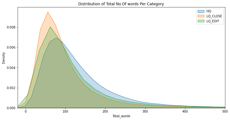
Now, let's see the distribution of a total number of words based on categories i.e. HQ, LQ_CLOSE, LQ_EDIT. Here, also we have used the same kdeplot to do the same. As we can see from the graph below, the distribution for each category looked almost similar and most of the questions have a total length of around 80–90 words in general.

plt.figure(figsize=(12,6))
p1=sns.kdeplot(df[df['Y']=='HQ']['Total_words'], shade=True,).set_title('Distribution of Total No.Of words Per Category')
p2=sns.kdeplot(df[df['Y']=='LQ_CLOSE']['Total_words'], shade=True)
p2=sns.kdeplot(df[df['Y']=='LQ_EDIT']['Total_words'], shade=True)
plt.legend(labels=['HQ','LQ_CLOSE','LQ_EDIT'])
plt.xlim(-20,500)

Now we will convert the target label into numeric values. Although there are various techniques to do so like one-hot encoding and label encoding but as there are only 3 categories( LQ_CLOSE, LQ_EDIT, HQ) we can simply use map function to do this task. You can see in the screenshot below that Y column values changed to numbers.

df['Y'] = df['Y'].map({'LQ_CLOSE':0,'LQ_EDIT':1,'HQ':2})
df.head()

Now, let's check if there are any null values or entries in our dataframe. It is good practice to check for the null values before they create any problem. We should perform this task in earlier stages.

df.isnull().sum()

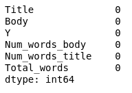
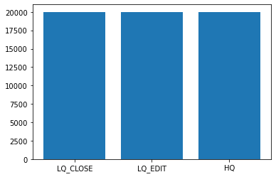
Now, we will plot the bar graph to show the number of questions for each label. We have used matplotlib.pyplot here and it turns out that each category have equal number of questions i.e. 20000

values = [len(df[df['Y']==0]),len(df[df['Y']==1]),len(df[df['Y']==2])]
plt.bar(['LQ_CLOSE','LQ_EDIT','HQ'],values)
plt.show()

Here, we combine the text of both title and body in one column named All_text. After that, we drop or delete the title and body columns.

df['All_text'] = df['Title']+' '+df['Body']
new_df = df.copy()
new_df = new_df.drop(['Title','Body'],axis=1)
new_df.head()

We have stored English stopwords( i.e. of the to etc.) in stop_words variable. After that, we have defined the function data_cleaning that takes a string(question) as an argument. In function, we first convert the data into lowercase, then remove any character other than alphabets. After that, the data is split and stored in a list called data. Then we remove the stopwords from the list and convert it back to a string using join. Finally, we return the cleaned data string.

from nltk.corpus import stopwordsstop_words = stopwords.words('english')def data_cleaning(data):
 data = data.lower()
 data = re.sub(r'[^(a-zA-Z)\s]','',data)
 data = data.split()
 temp = []
 for i in data:
 if i not in stop_words:
 temp.append(i)
 data = ' '.join(temp)
 return data

Here, we have just applied the data_cleaning function to all the values of All_text.

new_df['All_text'] = new_df['All_text'].apply(data_cleaning)
new_df['All_text']

We have imported train_test_split from sklearn.model_selection to split our data into training and testing set in the ratio of 5:1. As you can see in the screenshot below, training data consist of 48,000 questions and testing data is of 12,000 questions.

from sklearn.model_selection import train_test_splitx_train,x_test,y_train,y_test = train_test_split(new_df['All_text'],new_df['Y'],test_size=0.20)
print("X_train Size : ",x_train.size," Y_train Size : ",y_train.size)
print("X_test Size : ",x_test.size," Y_test Size : ",y_test.size)

Now, we will vectorize our data. Vectorization is the process of converting words or phrases into the corresponding vectors of real numbers used to find word predictions. And for this purpose, we have used TfidfVectorizer that stands for “Term Frequency — Inverse Document” Frequency which are the components of the resulting scores assigned to each word.

• Term Frequency: This summarizes how often a given word appears within a document.
• Inverse Document Frequency: This downscales words that appear a lot across documents.

Without going into the math, TF-IDF is word frequency scores that try to highlight words that are more interesting, e.g. frequent in a document but not across documents.

Look at this answer to understand more about TfidfVectorizer.

from sklearn.feature_extraction.text import TfidfVectorizer
vec = TfidfVectorizer()
x_train = vec.fit_transform(x_train)
x_test = vec.transform(x_test)

Now comes the part where we will train our model. For this purpose, I have used xgboost. Xgboost (Xtreme Gradient Boost) is a decision-tree based machine learning algorithm that also uses the gradient boost technique. It is one of the best and fast algorithms that performs well with unstructured data(images/text). But this is not enough to understand the inner workings of this algorithm. For this you will have to understand the concepts like bagging, boosting, decision trees. So, I will suggest you google more about xgboost after reading this article.

from xgboost import XGBClassifier
xgb = XGBClassifier()
xgb.fit(x_train,y_train)

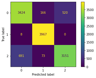
Our model is trained, now it's time to make predictions and check the accuracy of our model. Here, we have simply used predict() function provided with xgboost to make predictions and store them in the variable named predictions. For checking the performance of the developed model, we are using accuracy_score that calculates the % of correct predictions. ( We have used this performance matrix because we have a balanced dataset). The accuracy of our model is 87.56%.

from sklearn.metrics import accuracy_score,plot_confusion_matrix
predictions = xgb.predict(x_test)
acc = accuracy_score(predictions,y_test)
acc

For having even more information about our model and where its prediction goes wrong, we can plot the confusion matrix. As seen from the plot, for label 1(LQ_EDIT) it is almost correct, only 8 predictions were wrong. For labels 0,2(LQ_CLOSE, HQ) there were 686 and 764 wrong predictions respectively.

plot_confusion_matrix(xgb,x_test,y_test)

PREDICTION

Now let’s predict the quality label for one of the questions asked by the user. Here we have the title and body of the question for which quality is to be predicted.

NOTE:- I have cut the actual length of the body, full body is used for prediction which can be found in a notebook uploaded on Github.

title = "Pod install displaying error in cocoapods version 1.0.0.beta.1"
body = """<p>My podfile was working but after updating to cocoapods version 1.0.0.beta.1</p>\n\n<p>pod install displays following error</p>\n\n<pre><code>MacBook-Pro:iOS-TuneIn home$ pod install\nFully deintegrating due to major version update\nDeleted 1 'Copy Pods Resources' build phases.\nDeleted 1 'Check Pods Manifest.lock' build phases...."""

Here, we just follow the same procedure that we discussed earlier. Title and body are combined and data_cleaningfunction is used to clean the text. Vectorization is performed and then the prediction is done. The actual class for this question is HQ and the predicted class is 2(that corresponds to HQ).

All_text_testing = title+" "+body
All_text_testing = data_cleaning(All_text_testing)
All_text_testing_vector = vec.transform([All_text_testing])
prediction = xgb.predict(All_text_testing_vector)
prediction

CONCLUSION

So, we have successfully developed the machine learning model that predicts the quality of StackOverflow questions with an accuracy of 87.5%

FUTURE WORK

There are still some ways through which the performance of the model can be improved. Some of those are:-

• Using some advanced Deep Learning algorithms like RNN, BERT( as we have a large dataset deep learning algorithm might perform well)
• Using a more advanced data cleaning process. Here we are ignoring numeric data that might also help in improving the overall performance
• Using other techniques for vectorization like Word2Vec

The source code is available on GitHub. Please feel free to make improvements.

Thank you for your precious time.U+1F60AAnd I hope you like this tutorial.

Also, check my article on predict stock trend using deep learning

Join thousands of data leaders on the AI newsletter. Join over 80,000 subscribers and keep up to date with the latest developments in AI. From research to projects and ideas. If you are building an AI startup, an AI-related product, or a service, we invite you to consider becoming a sponsor.

Published via Towards AI