


Credit Risk Modeling — What if Models’ Prediction Accuracy Not High?
Last Updated on June 19, 2021 by Editorial Team
Author(s): Mishtert T
Real-world problems & Machine Learning
Credit Risk Modeling — What if Models’ Prediction Accuracy Not High?
What’s the best model performance?
This Article is intended to share concept and not methods or code.
One of the questions that I always get when I talk about credit risk modeling (Loan payment default, credit card payment default) is about the algorithms’ or models’ prediction limitations.
How can we implement a solution if the prediction probability is lower? How can we use the model or algorithm effectively for real-world problems?
Have chalked out what are all the available methods to predict the probability of default, while not getting into them detail since that’s not what this article’s intent is.
Let’s quickly take a look at some ways of how we can predict the probability of default.
Realization # 1:
All predictive models contain prediction errors. Accept it.
It may not possible to achieve a perfect score for real-word problems, given the stochastic nature of data and algorithms.
With that thought in mind, let’s move on.
Loan Default: Components
The main measure to make a decision before disbursing credit is Expected Loss, which consists of three components.
Expected Loss (EL):
- Probability of default (PD)
- Exposure at default (EAD)
- Loss given default (LGD)
How to compute Expected Loss
EL= (PD * EAD * LGD )
we’ll cover the probability of default-related information in this article.
Information Used for Decision Making:
Banks use various information before making a decision.
- Application information: Income, marital status, age, homeowner, etc…
2. Behavioral information: Account balance, historical payment timeliness, defaults, frequency of borrowing, etc…
Example Dataset
We’ll use an example dataset which contains information as shown below to explain a concept whenever there is a need in the below content.
> head(loan_dat)
  loan_status loan_amnt int_rate  grade  emp_length   home_ownership
1           0      5000    10.65   B         10           RENT
2           0      2400       NA   C         25           RENT
3           0     10000    13.49   C         13           RENT
4           0      5000       NA   A          3           RENT
5           0      3000       NA   E          9           RENT
6           0     12000    12.69   B         11           OWN
    annual_inc    age
1      24000      33
2      12252      31
3      49200      24
4      36000      39
5      48000      24
6      75000      28
Understanding the Data:
Perform Exploratory Data Analysis (EDA) to understand the dataset better.
- Outlier Management:
- Check for outliers using outlier detection methods (Univariate & Multivariate) — check these articles for quick understanding.
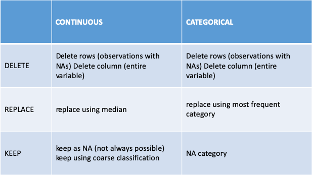
2. Missing data: Strategies
- Delete row/column (Not Recommended)
- Replace (Median Imputation)
- Keep NA (coarse classification, put the variable in “bins” )
Quick Cheat Sheet:
Some Methods to Create Models
We’re not going to discuss in-depth about how we’re going to create a model, but state a couple of ideas to explain the concept.
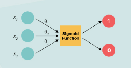
- A regression model with output between 0 and 1.
- We need to have a cutoff or threshold value to define if a prediction will be considered to be a default or non-default.
An example with “age” and “home_ownership” will look like below when solved will have a value of the probability of default.
P(loan_status = 1 | age =32 , home_ownership = Rent)
Decision Trees:
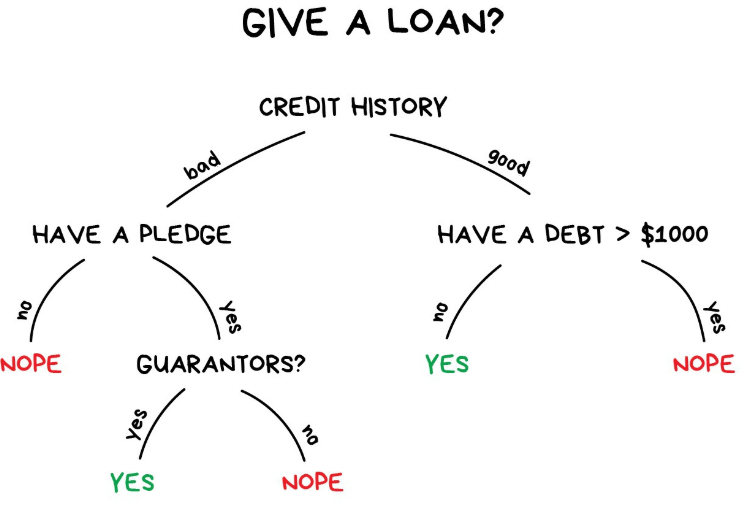
It’s hard to build a nice decision tree for credit risk data. The main reason is the unbalanced data.
To overcome unbalanced data,
- Undersampling or oversampling
- Accuracy issue will disappear
- Use only on the training set
- Changing the prior probabilities
- Including a loss matrix
Validate the models to see what is best!
Problems with large decision trees:
- They are too complex and not clear
- Overfitting happens when the model is applied to the test set
Pruning techniques should be considered
Some Measures
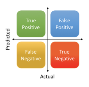
- Accuracy = (True Negative + True Positive) / (True Negative + False Positive + False Negative + True Positive)
- Sensitivity = True Positive/(False Negative + True Positive)
- Specificity = True Negative/(True Negative + False Positive)
- Precision = True Positive/(True Positive + False Positive)
- Recall = True Positive/(True Positive + False Negative)
- F1 score = (2 x (Precision x Recall)/(Precision + Recall))
How to use Accuracy, Precision, Recall Measures.
High Precision & High Recall: Good & Balanced Model
High Precision & Low Recall: Not good in detection, but accurate when it does
Low Precision & High Recall: Good detection capability, but chances of false positives high
Accuracy measures the number of correct predicted samples over the total number of samples and is not better measure for an imbalanced data.
It would make sense to use accuracy as a measure only if the class labels are uniformly distributed
Realization # 2:
No matter the number of loan applications rejected, there will still be debtors that default
Strategy:
Now that we realized that these models are never going to be 100% perfect, and how many ever applications are rejected based on the model, there will still be borrowers who will default.
The alternate solution to this problem is, we can use the model to decide how many loans the bank should approve if they don’t want to exceed a certain percentage of defaults.
Let’s assume a bank decides to reject 20% of new applicants based on the fitted probability of default. This means that 20% with the highest predicted probability of default will be rejected.
Cut off Value:
To get the cut-off value that would lead to the predicted probability of 1 (default) for 20% of cases in the test set, we should look at the 80% quantile of the predictions vector.
Having used this cut-off, we’ll know which test set loan applicants would have been rejected using an 80% acceptance rate.
Obtain the cut-off that leads to an acceptance rate of 80%
cutoff_point <- quantile(prob_default, 0.8)
Obtain the binary predictions. (Tag 1 if the predicted probability is > cutoff, else 0)
bin_pred <- ifelse(prob_default > cutoff_point, 1, 0)
If we take a look at the true status of the loans that would have been accepted using this cut-off and see what percentage of this set of accepted loans actually defaulted (which is also referred as bad rate)
accepted_loans <- test_set$loan_status[bin_pred == 0]
Obtain the bad rate for the accepted loans
bad_rate <- sum(accepted_loans) / length(accepted_loans)
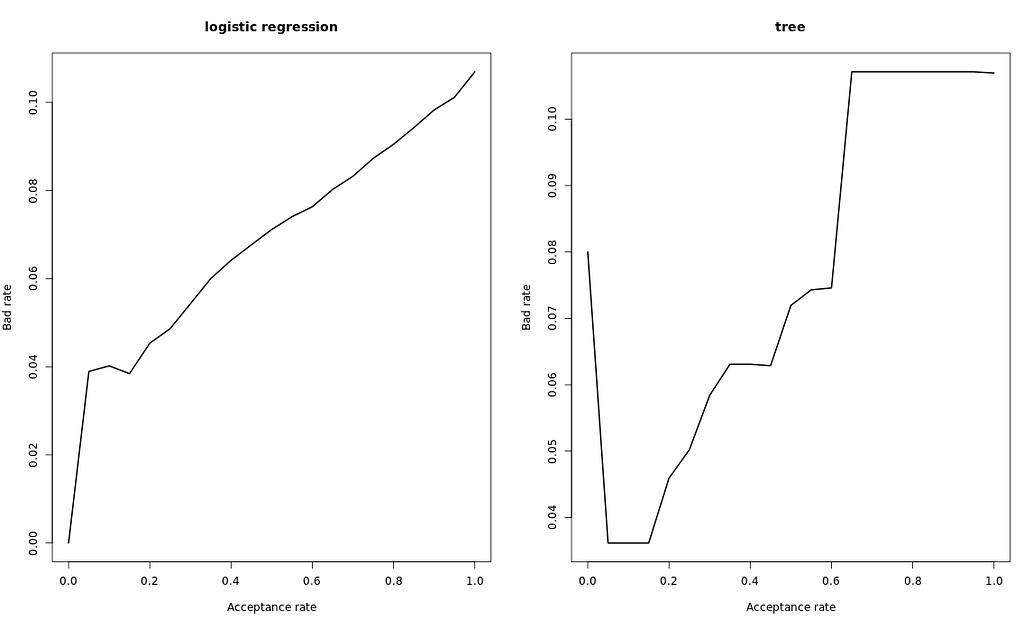
The strategy table and strategy curve
Repeating the calculations that we did in the previous exercise for several acceptance rates, we can obtain a strategy table.
This table can be a useful tool for banks, as they can give them a better insight to define an acceptable strategy.
Let’s assume we have two different models, the strategy table might look like this.
Strategy Table:


Strategy Curve:
Model Output Explanation to Non-Tech
What if the banks don’t want to go through this tough decision of having to choose acceptance rate or bad rate idea? What if, all they want is to know overall which is the best model?
Then building models with better AUC would be one way to explain. But it should be noted that better AUC doesn’t always solve our problems in the real world.
Pros:
- Measures how well predictions are ranked
- Measures the quality of the model’s predictions irrespective of what classification threshold is chosen.
Cons:
- If we require well-calibrated probability outputs, and AUC won’t tell us about that.
- In cases where the cost of false negatives vs. false positives is significantly important, minimizing one type of classification error may be critical. AUC will not be a helpful metric for this scenario.
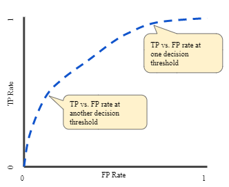
- ROC curve (receiver operating characteristic curve), a graph showing the performance of a classification model at all classification thresholds.
This curve plots two parameters: True Positive Rate & False Positive Rate
5. AUC (Area Under the ROC Curve), AUC measures the entire two-dimensional area underneath the entire ROC curve
- AUC ranges in value from 0 to 1.
- A model with100% wrong predictions will have an AUC of 0.0
- A model with 100% correct predictions will have an AUC of 1.0.
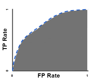
An AUC curve that’s is taller on left is usually a better model to say it in simpler terms.
Caution: Should be wary of false negative rate at all times if the problem statement is to reduce default.
Summary:
While building machine learning models with high AUC is the ideal way, this article is to let know someone who is unable to improve the model’s performance for whatever limitation that they can still try to couple their models with strategy curve and strategy table to answer some of the real-world problem questions.
Credit Risk Modeling — What if Models’ Prediction Accuracy Not High? was originally published in Towards AI on Medium, where people are continuing the conversation by highlighting and responding to this story.
Published via Towards AI
Towards AI Academy
We Build Enterprise-Grade AI. We'll Teach You to Master It Too.
15 engineers. 100,000+ students. Towards AI Academy teaches what actually survives production.
Start free — no commitment:
→ 6-Day Agentic AI Engineering Email Guide — one practical lesson per day
→ Agents Architecture Cheatsheet — 3 years of architecture decisions in 6 pages
Our courses:
→ AI Engineering Certification — 90+ lessons from project selection to deployed product. The most comprehensive practical LLM course out there.
→ Agent Engineering Course — Hands on with production agent architectures, memory, routing, and eval frameworks — built from real enterprise engagements.
→ AI for Work — Understand, evaluate, and apply AI for complex work tasks.
Note: Article content contains the views of the contributing authors and not Towards AI.
Related posts
Recent Posts


")