Combinatorial PurgedKFold Cross-Validation for Deep Reinforcement Learning

Author(s): Berend

Originally published on Towards AI the World’s Leading AI and Technology News and Media Company. If you are building an AI-related product or service, we invite you to consider becoming an AI sponsor. At Towards AI, we help scale AI and technology startups. Let us help you unleash your technology to the masses.

This article is written by Berend Gort & Bruce Yang, core team members of the Open-Source project AI4Finance. This project is an open-source community sharing AI tools for finance, and a part of the Columbia University in New York. GitHub link:

AI4Finance Foundation

Introduction

Our previous article described the Combinatorial PurgedKFold Cross-Validation method in detail for classifiers (or regressors) with regular predictions. This strategy allows for several backtest paths instead of a single historical one.

What qualifies as a valid empirical finding? A researcher will almost always identify a misleadingly profitable technique, a false positive, after many trials. Random samples include patterns, and a methodical search across a broad space of methods will eventually lead to discovering one that profits from the random data’s chance configuration¹. An investment strategy is likely to be fit for such flukes. The reason is that a set of parameters is tuned to maximize the performance of a backtest. “Backtest overfitting” is the term for this phenomenon.

A statistically correct improved analysis can be performed on multiple backtest paths, reducing the risk of negligible false discovery. Our previous article described what traditional Combinatorial Purged Cross-Validation could do for regular Machine Learning Backtests. The previous article:

The Combinatorial Purged Cross-Validation method

In this article, we write about an idea, not its execution. We need feedback on the ideation process and to create a discussion.

The novel idea is Combinatorial PurgedKFold Cross-Validation (CPCV) Deep Reinforcement Learning (DRL); CPCV DRL. There are some real concerns about the feasibility of this idea, and the solution might be problematic.

Applying these ideas in the DRL field is desired as the method is sample efficient in terms of backtests. Specifically, many coins have been only listed in the crypto field since ~ 2018. Therefore limited data is present to train and test a model. The rest of the rationale is present in our previous article.

Short intro: DRL for trading

Successful traders have their trading systems and can make sound judgments based on fundamental and technical analyses. However, due to: the information asymmetry of the crypto market, a lack of trading expertise, and human frailty, these analysis approaches are typically challenging to put into reality for ordinary investors. Reinforcement learning agents can learn effective policies for sequential choice problems and have surpassed humans in various tasks, for example, 2019 (!) Dota 2 World Championship. Just imagine it is already 2022.

So, can an RL agent train, learn from trading experiences, and automatically make good trading decisions? If so, what is the trading performance of such an agent?

DRL requires an environment of the crypto trading space that fully represents the actual exchange. This environment is used to train/test the DRL agents. For example, in Atari gaming, the state of the domain is defined as the last X continuous game screens in activities, and it is a complete depiction of the environment. Unlike the deterministic and noise-free environment described above, crypto prices are known to be volatile, and the trading environment changes with time.

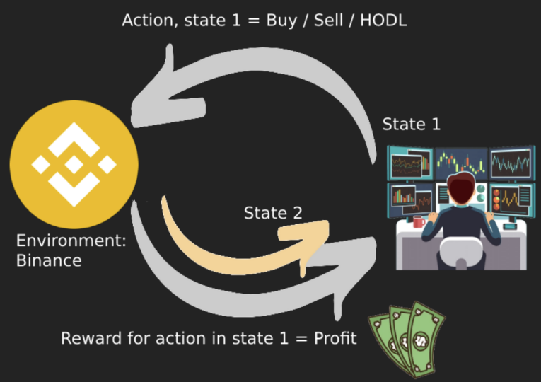
In crypto trading, the state vector could be all of the features from the dataset and the information about the trading account. For example: how much cash is in the account, the technical indicators, and the amount of crypto the account holds from the tradeable pairs. Figure 1 shows how a DRL could be profitable in a cryptocurrency exchange. There is a state (trader) of which an action can be performed (buy/sell/hold). The environment, in this case, is the trade market, and the reward system is the profit.

OK, that was the quick summary. From here, we will assume the reader knows about DRL (trading) algorithms and wants to backtest a strategy. In the next section, we will shortly describe how to perform a ‘single’ backtest.

Traditional DRL Backtesting

Benchmark

The goal of the trading bot is to maximize portfolio value whilst hedging risks like market crashes. Therefore, the bot needs to be benchmarked; a valuable comparison with other trading strategies.

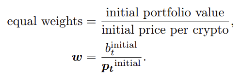
Equal weight (EQW) is a proportional measurement technique that assigns equal weight to each cryptocurrency in a portfolio, index, or index fund. In straightforward terms: if the trading account has 1 million US dollars and there are 4 cryptocurrencies of interest, distribute 250k to each coin, which is called an EQW-portfolio.

Thus, when measuring the group’s performance as a whole, the crypto wallets of the smallest firms are assigned the same statistical importance, or weight, as those of the biggest crypto wallets. The initial portfolio value is distributed according to:

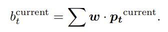
After that, the current value of the portfolio is computed as:

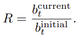
The return of this strategy is then the final portfolio value divided by the initial portfolio value. Thus, the equal-weight investment strategy is equivalent to distributing the cash equally to each crypto trading pair and leaving it there.

Sharpe Ratio

The Sharpe ratio is a financial statistic that compares the performance of an investment (e.g., a crypto investment) to that of a risk-free asset after risk is taken into account. It is defined as the difference between the investment’s returns and the risk-free rate of return, divided by its standard deviation (i.e., its volatility). It is the increased return that an investor obtains due to an increase in risk. The Sharpe ratio is one of the most widely used methods for calculating risk-adjusted return. The formula for the Sharpe ratio is as follows:

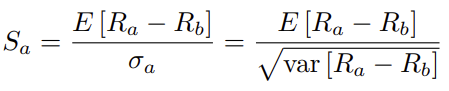
R(a) is the asset return, and R(b) is the risk-free return. E [R(a) − R(b)] is the expected value of the excess of the asset return over the benchmark return, and σ(a) is the standard deviation of the asset excess return. The DRL agent’s goal is to maximize return whilst minimizing risks. Therefore the Sharpe ratio will be used as a target for hyperparameter optimization.

Model Selection

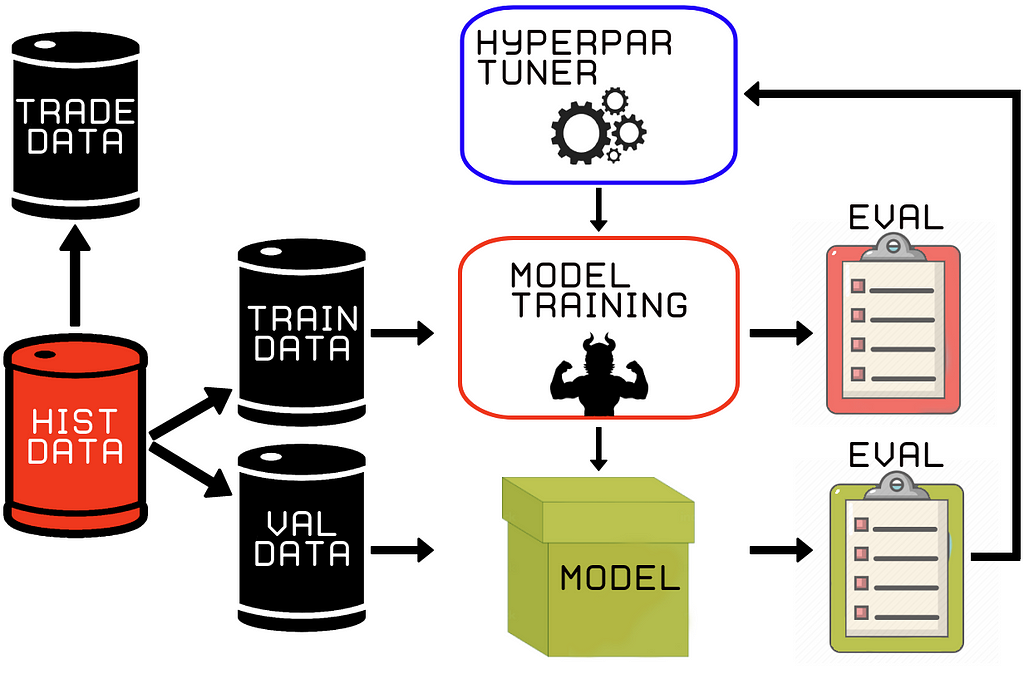
The historical dataset exists for three different periods:

• Training data (in-sample, IS)
• Validation data (in-sample, IS)
• Trade data (out-of-sample, OOS)

Figure 2, IS periods consist of data for training and validation stages. During hyperparameter optimization, the train and validation sets are used to obtain a well-trained model. After for example 100 trials, the model with the highest Sharpe ratio is selected. The evaluation of this selection process is displayed in Figure two by the yellow ‘eval’ checkpoint.

If the Sharpe ratio of the trained model is the highest so far during this particular optimization, the model is saved for the next phase (model simulation).

Model Simulation Example

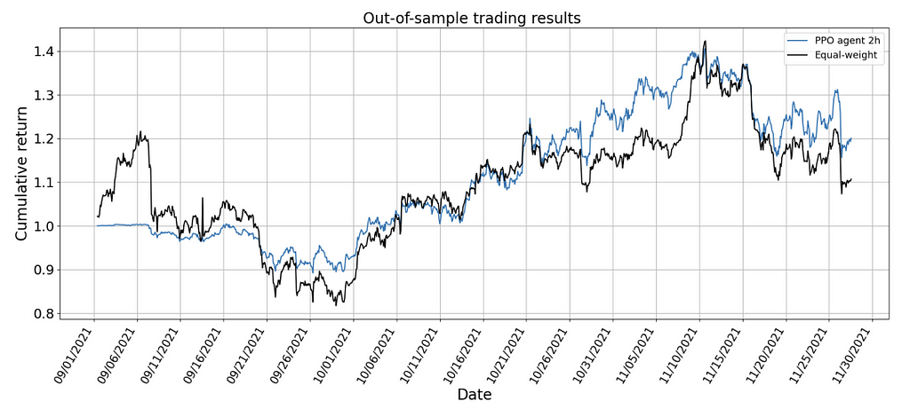
After that, the out-of-sample trade data is used to backtest the real-time trading performance (Figure 3) of the ‘best’ agent. Thus, the DRL agent is not trained or validated on the OOS data to produce results assumed as real-time trading performance.

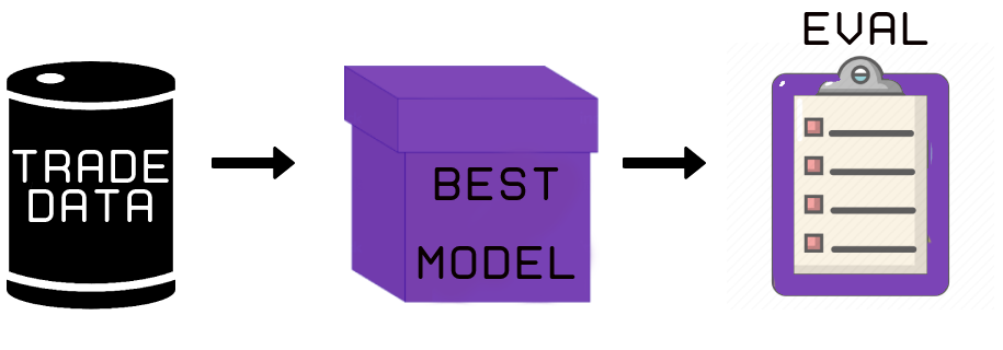
In this stage, the actual profitability of the agent is computed. There are five main metrics to evaluate the results.

• Cumulative return: subtract the portfolio’s final value from its starting value and divide it by the initial value.
• Annualized returns: they are the geometric mean of the strategy’s annual earnings.
• Annualized volatility: the annualized standard deviation of the portfolio return.
• Sharpe ratio: subtract the annualized risk-free rate from the annualized return and then divide by the annualized volatility.
• Max drawdown: The highest point value is subtracted by the lowest point in the time frame.

Explanatory Analysis and Results

The results are given in Figure 4. The 1m, 5m, …, 2h, 4h are the candle-widths of the crypto data. These exact results are obtained by running the hyperparameter tuner for 100 trials on each timeframe, and then running the Model Simulation process.

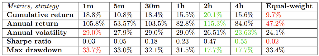
Figure 4 demonstrates that the DRL agents outperform the equal-weight benchmark in multiple perspectives. As can be seen from Fig 4, every single DRL agent outperforms the benchmark in terms of the Sharpe ratio. The Sharpe ratio for the equal-weight strategy is 0.02, compared to 0.47 for the 2h and 0.55 for the 4h. The annualized return of the agent is significantly higher as well. The equal-weight strategy manages 47.2%, which is in this particular timeframe worse than the others. Therefore, these findings demonstrate that the proposed DRL agent can effectively develop a trading strategy that outperforms the baseline.

Based on Figure 4, either the 2h or 4h timeframe seems to be best. The excess returns on the 2h timeframe are significant enough to ignore the decrease in annual volatility. Therefore, the 2h model is selected and will be deployed on the OOS trade data. Figure 5 shows the selected model for deployment versus the benchmark, to visually show that it is less volatile, has less drawdown, less risk, and increased returns.

The Backtest Fluke

• We repeat:

A researcher will almost always identify a misleadingly profitable technique, a false positive, after many trials. Random samples include patterns, and a methodical search across a broad space of methods will eventually lead to discovering one that profits from the random data’s chance configuration¹. An investment strategy is likely to be fit for such flukes. Especially when a set of parameters is tuned to maximize the performance of a backtest. “Backtest overfitting” is the term for this phenomenon.

• Concerning the previous section:

We suspect there is an issue in the Model Selection part of the proposed backtest strategy. As stated, we have performed 100 hyperparameter trials on the validation results and selected the model that delivers the highest Sharpe ratio for that time frame. The more trials we do, the higher the probability that we just got ‘lucky’ on the validation set.

Let us move on to the novel idea, which reduces the risk for the hyperparameter optimizer to find a ‘lucky’ result. We do not want to get lucky; we want to be calculated.

The novel idea: CPCV DRL

If the reader has not read our previous article yet, we advise you to read that first. In that article, we describe the Combinatorial PurgedKFold Cross-Validation method for traditional machine learning. Article:

The Combinatorial Purged Cross-Validation method

We present the main result from the CombPurgedKFoldCV method (Figure 6).

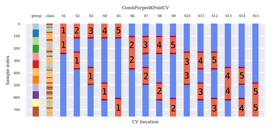
For each data split, it is the same story as with traditional cross-validation: we train on the blue data and test on the read data. However, in the next section, we present how Combinatorial Purged K-fold Cross-Validation could be applied to DRL.

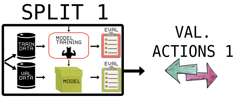
See Figure 7; we save all the actions during the validation stage instead of looking only at the Sharpe ratio for one split. Thus, we train and validate as usual, except we look at the best-predicted actions of the DRL agent, which represent the basic trading strategy.

Note that we have highlighted validation groups now (Figure 2, Figure 6).

• Split 1 || train : (G3, S1), (G4, S1), (G5, S1), (G6, S1) || validation : (G1, S1), (G2, S1) || → DRL agent 1 → actions y(1,1), y(1,2) on (G1, S1), (G2, S1)
• Split 2|| train : (G2, S2), (G4, S2), (G5, S2), (G6, S2) || validation : (G1, S2), (G3, S1) || → DRL agent 2 → actions y(1,2), y(3,2) on (G1, S2), (G3, S2)
• …….
• Split 15|| train : (G1, S15), (G2, S15), (G3, S15), (G4, S15) || validation : (G5, S15), (G6, S15) || → DRL agent 15 → actions y(5,15), y(6,15) on (G5, S15), (G6, S15)

DRL itself is a walk-forward algorithm; it is a sequential algorithm. So for each split, the DRL agent will do a walk-forward path through the validation data to get actions. We save these actions in a matrix corresponding to the groups and splits presented in Figure 6.

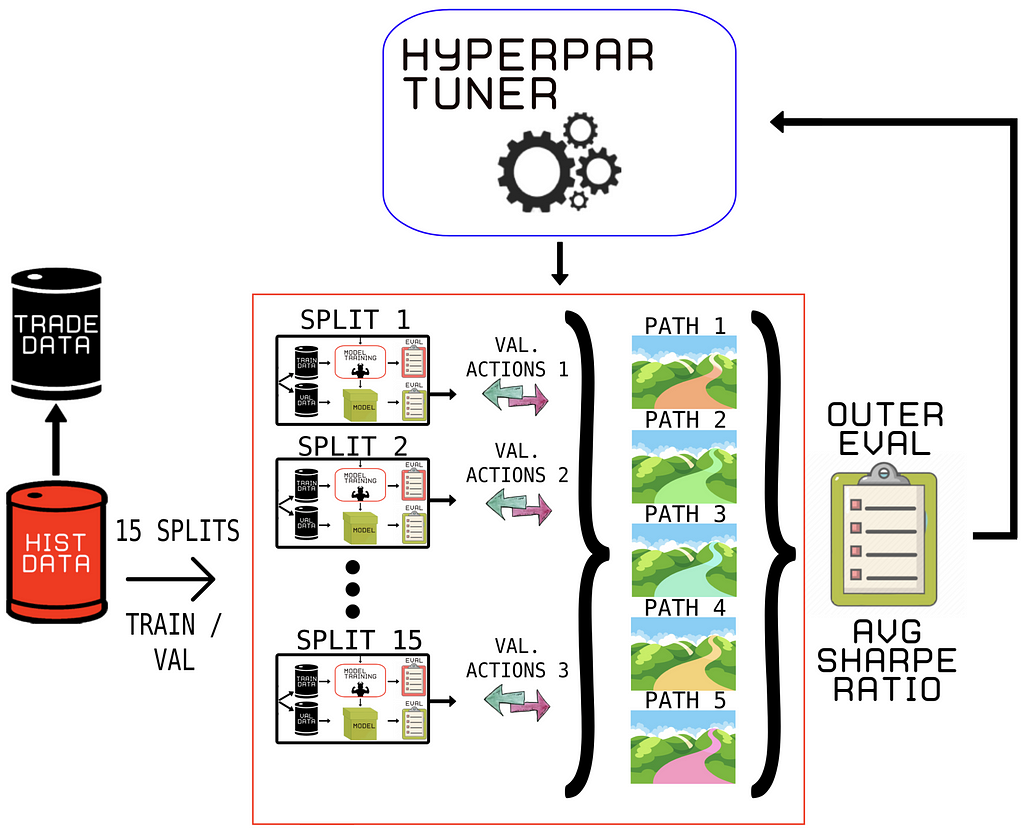
See Figure 8 for the new Model Selection process. First, we choose which part to use for the in-sample part (train and validation data) and which data we want to do the final backtest on (trade data). After that, we train the DRL agent on the train data of each split (Figure 6) and evaluate each agent in a walk-forward manner on the validation data, producing actions at each data point.

These actions at each data point are stored according to Figure 6. Therefore, we can see the actions produced by the DRL agent in the validation stage as ‘predictions’ (like in the previous article). These ‘actions/predictions’ represent the basic trading strategy produced for that time period. Finally, just like in the previous article, we can form 5 unique paths on which we can backtest our strategy.

In our hyperparameter optimizer, we use the average Sharpe ratio of all of the 5 backtest paths as the final evaluator of the optimization loop. We have significantly reduced the risk of overfitting a single validation path even after many trials!

Because researchers will choose the backtest with the highest estimated Sharpe ratio, even if the Sharpe ratio is zero, WF’s high variance leads to faulty findings. That is why, when performing WF backtesting, it is critical to account for the number of trials.

Due to CPCV DRL, it is now possible to calculate the Family-Wise Error Rate (FWER), False Discovery Rate (FDR), or Probability of Backtest Overfitting (PBO)². In contrast, CPCV derives the distribution of Sharpe ratios from a large number of paths, j = 1, … , 𝜑. The average Sharpe Ratio of the distribution is the mean E[{y i,j } (j=1,…,𝜑 )] = 𝜇 and variance 𝜎²[{y i,j } (j=1,…,𝜑 )] = 𝜎²(i).

CPCV, on the other hand, calculates the Sharpe ratio distribution from a large number of pathways, j = 1, … , 𝜑. The mean E[{y i,j} j=(1,…, 𝜑)] =𝜇 and variance 𝜎²[{y i,j }(j=1,…, 𝜑)] = 𝜎²(i) are the average Sharpe Ratios of the distribution. The sample mean of CPCV pathways has a variance of:

Where 𝜎²(i) is the variance of the Sharpe ratios across paths for strategy i, and α(i) is the average off-diagonal correlation among {y i,j } (j=1,…,𝜑). CPCV leads to fewer false than CV and WF because α(i)< 1 implies that the variance of the sample means is lower than the variance of the sample. Imagine we have (almost) no correlation between the backtest paths to put matters into perspective. If no correlation is assumed, then α(i) ≪ 1. The Equation above will reduce to:

As a result, the lower the variance of CPCV, the statistically valid Sharpe ratio E[y(i)i] will be reported with zero variance in the limit of φ→∞ (amount of paths to infinity). Because the strategy is chosen from i = 1,…, I will have the highest statistically valid Sharpe Ratio, there will be no selection bias.

Finally, the more path’s the less the variance will become and the closer we get to the statistically valid Sharpe ratio. However, the amount of paths is upper bounded by the amount of available data. Still, for a large enough number of paths 𝜑, CPCV could make the variance of the backtest so small as to make the probability of a false discovery negligible.

Conclusion

In the previous article, the Combinatorial Purged Cross-Validation method is explored. Then, in this article, a suggestion is made to extend this method to the DRL domain. The issues regarding traditional WF methods are summarized. After that, an introduction to DRL for trading is given. Subsequently, an overview of traditional DRL backtesting is provided, which is a complete backtesting analysis. Finally, the novel idea of doing a Combinatorial Purged Cross-Validation with DRL is presented in a possibly feasible manner. The method could bring the Model Selection process closer to the statistically valid Sharpe Ratio.

Thanks for getting to the bottom of “Combinatorial PurgedKFold Cross-Validation for Deep Reinforcement Learning”!

~ Berend & Bruce

Reference

1. Bailey, D. and Lopez de Prado, M., 2014. The Deflated Sharpe Ratio: Correcting for Selection Bias, Backtest Overfitting and Non-Normality. SSRN Electronic Journal.

2. Prado, M. L. de. (2018). Advances in financial machine learning.

---

Combinatorial PurgedKFold Cross-Validation for Deep Reinforcement Learning was originally published in Towards AI on Medium, where people are continuing the conversation by highlighting and responding to this story.

Join thousands of data leaders on the AI newsletter. It’s free, we don’t spam, and we never share your email address. Keep up to date with the latest work in AI. From research to projects and ideas. If you are building an AI startup, an AI-related product, or a service, we invite you to consider becoming a sponsor.

Published via Towards AI