Building Feedforward Neural Networks from Scratch

Author(s): Nicolò Tognoni

Originally published on Towards AI the World’s Leading AI and Technology News and Media Company. If you are building an AI-related product or service, we invite you to consider becoming an AI sponsor. At Towards AI, we help scale AI and technology startups. Let us help you unleash your technology to the masses.

Everything you need to know about Feed Forward Neural Networks (FFNNs). From learning what a Perceptron is, to Deep Neural Networks, to Gradient Descent, and Backpropagation.

This article will give you a general idea of what Feed Forward Neural Networks (FFNNs) are. Starting from the basics, like what a Perceptron is, arriving at Backpropagation.

In the last part of the article, there’s a tutorial on how to build an FFNN in Python using Tensorflow.

Since many topics covered are too big to be completely explained in just one article, there’s a section at the end of many paragraphs called “Recommended Reading” where you can find really helpful articles to learn more on those topics.

Before diving into the article, I just want to tell you that if you are interested in Deep Learning, Image Analysis, and Computer Vision, I encourage you to check out my other article:

Train StyleGAN2-ADA with Custom Datasets in Colab

Table of contents

1. Neural Networks
2. Feed Forward Neural Networks (FFNNs)
3. Why Layers?
4. Cost Function
5. Gradient Descent
6. Backpropagation
7. Tutorial — Building a Feed Forward Neural Network
8. Conclusions
9. References

1. Neural Networks

Neural Networks, also known as Artificial Neural Networks (ANNs) or Simulated Neural Networks (SNNs), are a subset of machine learning and are at the heart of deep learning algorithms. Their structure is inspired by the neurons in the human brain and the way they work by sending electric charges to one another.

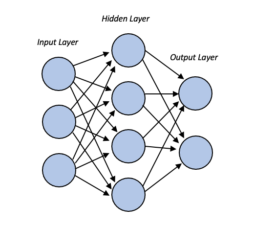
They are composed of node layers: an input layer, one or more hidden layers, and an output layer. Nodes are connected to each other, and for each connection, there is associated a weight. If the output of the node is greater than a certain threshold, then the node is activated, and the data gets passed to the next layer.

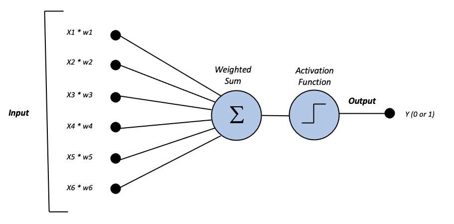
To understand how Neural Networks work, we first have to understand a type of artificial neuron called Perceptron (image above). It’s composed of four parts: one input layer, weights and bias, net sum, and activation function.

• The inputs, x1, x2, …, are passed to the Perceptron. Both the inputs and the single output are binary.
• The weights, w1, w2, …, are a representation of how the respective input is important to the output in the network. They’re composed of real numbers.
• The inputs x are multiplied by their weights w. Then, you sum all the values and pass the result to the activation function.
• The activation function determines the output value to be either 0 or 1 based on a determined threshold value.

The perceptron uses the Step Activation Function that is either 0 when x < 0, and 1 if x ≥ 0.

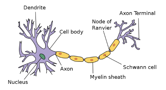
The same thing happens with neurons in our brain: Dendrites collect charges from synapses, both inhibitory and excitatory. The cumulated charge is released (neuron fires) once a threshold is passed.

2. Feed Forward Neural Networks (FFNNs)

Feed Forward Neural Networks (FFNNs), also known as Multilayer Perceptrons (MLPs) is composed of an input layer, an output layer, and many hidden layers in the middle. The idea is that you transform the signal by the combination of many nonlinear functions.

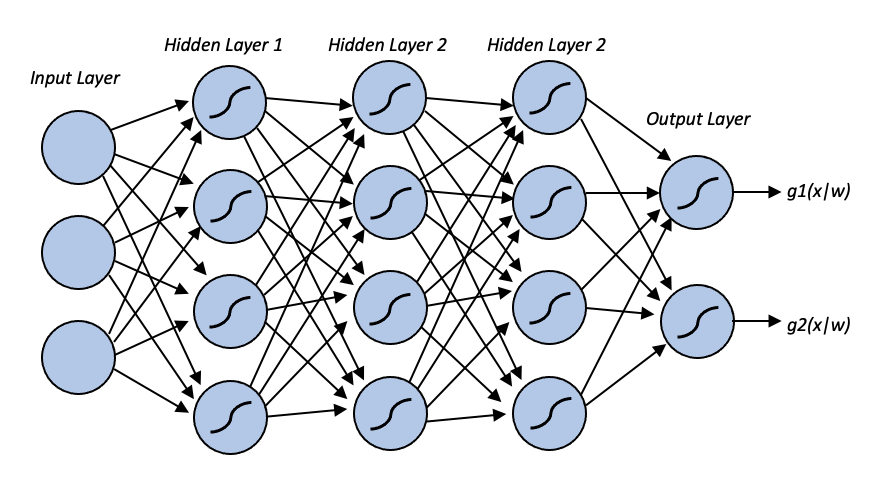
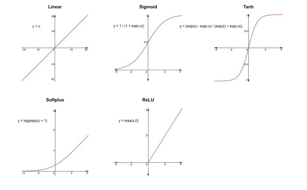
You can choose many activation functions, but the most popular non-linear functions are Sigmoid and ReLU. Here there are some examples of activation functions frequently used in Neural Networks:

The output layer in FFNNs is composed of as many neurons as the categories we want to predict.

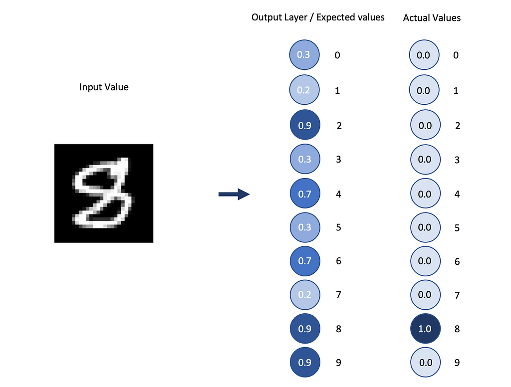
If we want to predict handwritten digits, we’ll have 10 categories, one for each digit (0, 1, 2, …, 9), the output layer will represent how much the system thinks an image corresponds to a given category, so the probability.

3. Why Layers?

Why do we use many layers in neural networks?

The activation of each neuron in a certain layer has an influence on the activation of each neuron in the next layer and so on.
Some connections could be stronger than others, indicating that some neurons have a stronger influence in the network than others.
This is at the base of backpropagation, that we’ll see later.

Layers break problems into small size pieces.

If we want to recognize a handwritten number, the problem will be divided into smaller pieces.

• To recognize an 8, we first want to recognize the component of the 8, for example, that is composed of two circles, one on top of the other.
  But then the next question is: how do you recognize a circle in the first place?
• To do so, you could, for example, say that a circle is composed of four small edges.
  Even then, we could go on and ask ourselves, how do you recognize an edge? And so on…

We could think that each layer of the neural network solves each one of these problems:

• The first layer recognizes small edges and passes this information to the second layer.
• The second one, given this information, recognizes two circles by summing the small edges together.
• It then passes this information to the third layer that recognizes two circles, one on top of the other.
• We finally arrive at the output layer that, based on the information it receives from the network, gives a high probability that the input is an 8.

This is an oversimplification of the process, but it gives you a good understanding of how a real neural network works.

Layered structures of neural networks allow them to break down difficult problems into smaller and easier problems.

4. Cost Function

But how do we train a Neural Network?

To have an idea of how it works, we first need to understand how we reduce errors in linear regression.

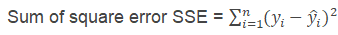
In linear regression, to optimize the function and reduce the errors, we use the sum of squared errors, the difference between the predicted value and the sample mean.

This is the same principle as the one of the Loss function or Cost function, a function whose objective is to evaluate how our algorithm is performing and how good or bad our model is.

• The Loss function computes the errors of a single training example.
• The Cost Function computes the average of the loss functions for all the examples.

The goal is to reduce the errors between the actual and the predicted values and so to minimize the Cost Function.

There are many loss functions to choose from. The most common are:

• Binary Cross-Entropy
• Categorical Cross-Entropy
• Mean Squared Error
• Logarithmic Loss

5. Gradient Descent

Now we know how bad or good our model is, but this is not useful information taken by itself. How can we improve our model?

To do so, we want to take our Cost Function and find an input that minimizes the output of the function, the point where the errors are the minimum. We want to find the weights and biases that make the cost as small as possible.

To do so, in the case of non-linear functions, we have to use gradient descent, the most common way to optimize neural networks. It’s used to find the minimum value for a function.

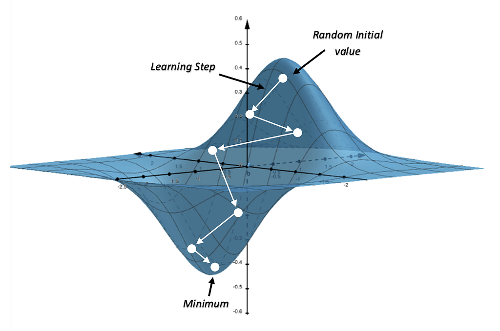
The gradient descent is based on a convex function and behaves as follows:

• The starting point is a random point
• From that starting point, we find the derivative, the slope of the curve at a given point, to understand how steep the function is increasing or decreasing. We expect the slope to decrease over time as we approach a minimum point.
• The gradient tells us in which direction the function is increasing. Since we want to reach a minimum, we want to proceed in the direction where the function is decreasing or the opposite of the gradient.
• To calculate the next point, we use the gradient of the current position, then multiply it by the learning rate, and finally subtract the obtained value from the current position.

This process can be written as:

a n+1 = is the next position of our climber
a n = represents his current position
Minus (-) = indicates the minimization part of gradient descent
ɣ = is the learning rate
∇F(a n) = the gradient term indicates the direction of the steepest descent

This process continues until it finds a minimum in the function.

There are three types of gradient descent algorithms:

• Batch Gradient Descent: It sums the error for each point in the training set, but only after all training examples have been evaluated is the model updated. This process is called a training epoch.
  Batch gradient descent needs to store all of the data in memory, which could cause a long processing time for large datasets.
  Moreover, while it produces a stable error gradient and convergence, it could get stuck in a local minimum and not find the global one.
• Stochastic Gradient Descent: This type of Gradient runs a training epoch for each example. It then updates the parameters of each example one at a time.
  The advantage of this type of gradient descent is that you only need to store one training example per time and not all the data, so you don’t need a lot of memory, and the process could be faster.
  However, it may result in a loss of computational efficiency compared to the former, and the continuous updates can result in noisy gradients.
• Mini-batch gradient descent: It combines concepts from the first two. It divides the dataset with the training examples into sample batch sizes. It then performs updates on each of those batches.

Recommended Reading:
If you want to learn more about Gradient Descent and the math behind it, I highly encourage you to read this article:

Gradient Descent Algorithm — a deep dive

6. Backpropagation

Backpropagation is the most fundamental building block in a neural network, firstly introduced in the 1960s.

The backpropagation tries to minimize the cost function by adjusting the weights and biases of the network based on the gradient calculated with the gradient descent.
What tells us how sensitive the cost function is to the corresponding weight and bias is the magnitude of every component of the gradient.

In the beginning, the network is not yet trained, so the outputs are random. To make it better, we need to change the activations of the last layer to make better predictions.
However, we can’t directly change the activations, we can only change the weights and the biases, so we’ll have to adjust those to improve the output.
What is helpful is to see which adjustments we would like to do to the activations to make better predictions.

Let’s give an example to make things clear.
If we want to recognize handwritten digits (like the MNIST database), we want to see, for a determined example (like the number 8), which activations we want to change to recognize the digit as an 8 effectively. In other words, when the neural network sees an 8, we want the probability of being an 8 in the output layer of the model to be the highest.

Some values in the output layer (consisting of 10 neurons, one for each category: 0, 1, 2, …, 9) will have to be increased, while others will have to be decreased.
More important is the magnitude of these changes for each neuron — how far the output of each neuron (predicted value) is from the actual value it should have.

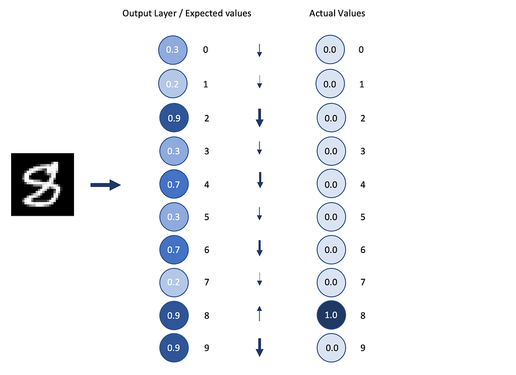
Let’s remember that the activation value of each neuron is the weighted sum of all activations from the previous layers, plus a bias.

If we want to increase an activation, we can either increase the weights, change activations from the previous layer, or increase the bias, but we can only change the weights and biases.

Recommended Reading:
You should now have a solid foundation on backpropagation, but if you would like to explore the topic further, I encourage you to read this article:

3Blue1Brown – Backpropagation calculus

7. Building a Feed Forward Neural Network

Let us now put into practice what we have learned so far.

In this tutorial, we’ll create with TensorFlow a simple FFNN with one input layer, one hidden layer, and an output layer.

We’ll use the MNIST Dataset of handwritten digits, which consists of 60,000 examples and a test set of 10,000 examples. Each example is a 28×28 grayscale image associated with a label from 10 classes.

Loading the Data

The first step is loading the data.
Since MNIST is one of the most popular datasets for image classification, it’s already in Keras (TensorFlow), and to load it, we can directly use Keras API.

Model

The next step is creating the model FFNN.

We’ll create a simple FFNN composed of an input layer, one hidden layer, and an output layer.

The first thing to do is to create a Flatten layer of size 28×28 (784) that corresponds to the width times the height of the images in the dataset.
This is done so that every pixel of the image is represented in the model.

The hidden layer is a dense layer composed, in our case, of 1000 neurons.

Finally, the output layer is another dense layer, and it needs to be of the same size as the number of categories in the dataset that we want to predict, 10 in the MNIST dataset, one for each number (0, 1, 2, …, 9)

To create the model, we use Keras Sequential API.

Training

The last step is to compile the model.
To do this, we need to choose an Optimizer, a Loss Function, and the Metrics we want to be shown during training to get an idea of how the model is behaving.

As the Optimizer, we’ll use the “SGD” that stands for Stochastic gradient descent.

We’ll use the Sparse Categorical Crossentropy for the Loss Function.

To understand how our model is performing, we’ll use the Accuracy of the model on both the training set and the test set.

The last step is to use the .fit method to begin training the model.
In this step you must choose the training set and the validation set, as well as the number of epochs for which you want the model to run.

Valuation

From the training, we get this output:

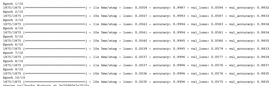
We can see that the accuracy both on the training set and the validation set is really high at around 99% and 98%.

Even if the model has only three layers and runs for 10 epochs, the predictions generated are really accurate.

8. Conclusions

In this article, we started from the basics: we learned what Neural Networks are. We understood what a Perceptron is and its components.

We then moved to Feed Forward Neural Networks and their activation functions. We then deep-dived into Gradient Descent and Backpropagation.

In the last part of the article, we built an FFNN from scratch using python, and we trained it using MNIST Dataset.

If you found this article helpful, check out my profile on Medium and connect with me on LinkedIn!

9. References

[1] Ian Goodfellow, Yoshua Bengio and Aaron Courville, Deep Learning (2016), The MIT Press

[2] Parul Pandey, Understanding the Mathematics behind Gradient Descent. (2019), Medium

[3] IBM Cloud Education, What is Gradient Descent? (2020), IBM

[4] Grant Sanderson, What is backpropagation really doing? (2017), 3Blue1Brown

---

Building Feedforward Neural Networks from Scratch was originally published in Towards AI on Medium, where people are continuing the conversation by highlighting and responding to this story.

Join thousands of data leaders on the AI newsletter. It’s free, we don’t spam, and we never share your email address. Keep up to date with the latest work in AI. From research to projects and ideas. If you are building an AI startup, an AI-related product, or a service, we invite you to consider becoming a sponsor.

Published via Towards AI