Bayesian Inference in Python

Author(s): Shanmukh Dara

Originally published on Towards AI the World’s Leading AI and Technology News and Media Company. If you are building an AI-related product or service, we invite you to consider becoming an AI sponsor. At Towards AI, we help scale AI and technology startups. Let us help you unleash your technology to the masses.

Probability

Discover the distinction between the Frequentist and Bayesian approaches.

Uncertainty is the only certainty there is, and knowing how to live with insecurity is the only security — John Allen Paulos

Life is uncertain, and statistics can help us quantify certainty in this uncertain world by applying the concepts of probability and inference. However, there are two major approaches to inference:

• Frequentist (Classical)
• Bayesian

Let’s look at both of these using the well-known, and simple Coin flip example.

What can we say about the fairness of a coin after tossing it 10 times and observing 1 head and 9 tails?

Although 10 is small sample size for determining the fairness of a coin, I chose it because collecting a large number of samples in real life can be difficult, especially when risk and opportunity costs are high.

Frequentist Inference:

This is the one that is commonly taught in colleges and frequently used in industry, but it is not without criticism.

Basic idea: The frequentist method computes a p-value, which is the probability of observing an outcome at least as extreme as the one in our observed data, assuming the null hypothesis is true.

The null and alternative hypothesis, in this case, would be:
H0: The coin is fair
H1: The coin is biased

Assuming the coin is fair, we calculate the probability of seeing something as extreme as 1 head. That is 1 head, 0 heads, and 9 heads and 10 heads on the other side. Adding all four results in a probability of 0.021.

from scipy.stats import binom

binom.pmf(k=9, n=10, p=0.5)  + binom.pmf(k=10, n=10, p=0.5) +binom.pmf(k=0, n=10, p=0.5)+binom.pmf(k=1, n=10, p=0.5)

So, at 5% significance, we can confidently reject the null hypothesis and conclude with 95% certainty that the coin is biased.

Everything appears to be in order so far, and we’ve established that the coin is biased. So, what’s the issue?

Assume the observer was dissatisfied with the answer and went on to observe ten more samples with the same coin. Will he draw the same inference about the coin? Not necessarily. This time, he could see 5 heads and 5 tails and conclude that the coin is not biased. As a result, we’re having trouble reproducing the same results under the same conditions.

In addition, We’ll never understand how reasonable our null hypothesis is because we assumed it was true — You can make an absurd claim and then design an experiment to reject or accept the null hypothesis.

So, do we have any other robust methods that can overcome these constraints?

Bayesian Inference:

Bayesian inference takes a very different viewpoint from the frequentist approach, instead of estimating a single population parameter from the observed data, we characterize them with entire probability distributions which represent our knowledge and uncertainty about them.

We start with prior probability which represents what we know about the parameters before seeing data, then we make observations, and depending on them we update the prior into posterior using Bayes’ rules.

So let’s start with the Bayes’ rule:

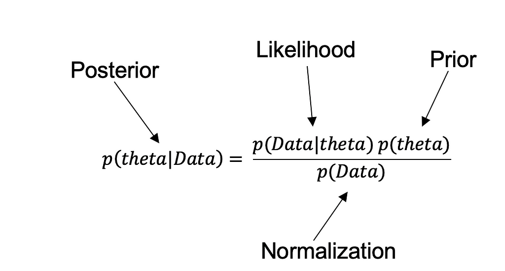
Theta in the equation is the success of the experiment, Data here is the observed data from experimentation, let's understand each term in the equation

· P(theta) — also called prior — it is the probability of success before seeing the data, this comes

· P(theta | Data) — also called posterior — it is the probability that Hypothesis is true after considering the observed data

· P(Data | theta) — also called likelihood — it is the evidence about Hypothesis provided by the data

· P(Data) — also called Normalization — is the total probability of the data taking into account all possible hypotheses

Inference about an incident can be offered in three ways.

1. Entirely based on your prior experience, without any observed data, — i.e. based on p(theta) a.k.a prior, which is a non-statistician approach to things.
2. The second way is the frequentist method, in which we anticipate how rare it is to observe this outcome if the hypothesis is true, i.e. p(data | theta) a.k.a likelihood, which means we are simply relying on observed data and nothing else.
3. Finally, we have Bayesian inference, which uses both our prior knowledge p(theta) and our observed data to construct a distribution of probable posteriors. So one key difference between frequentist and Bayesian inference is our prior knowledge, i.e. p (theta).

So, in Bayesian reasoning, we begin with a prior belief. Then we examine the observed data, allowing each data piece to alter our previous understanding slightly. The more data we observe, the further we can stray from our initial beliefs. This procedure finally results in a posterior belief.

But there’s a catch: if prior refers to our previous understanding, doesn’t this add experimenter’s bias? What if we obtain different results because of different priors? These are all fair questions, however, the prior is an important part of Bayesian inference, and one should ensure that his prior is relevant.

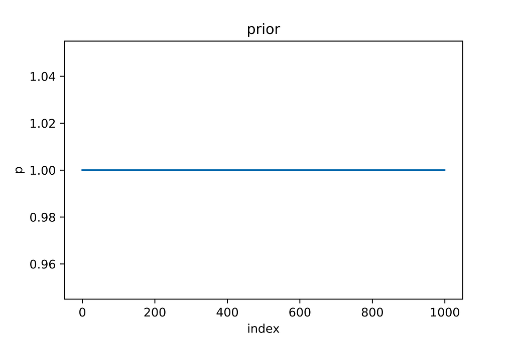
So, to compute the posterior precisely, we need a prior and a likelihood for the hypothesis, but in most experiments, the prior probabilities on hypotheses are unknown. In this scenario, we can assume that the prob(theta) is uniformly distributed between 0 and 1.

Let’s return to our coin flip example:

p(theta) — the probability of success (heads) — before seeing data, what is the probability of success— as we don’t have any prior knowledge of the coin, we assume it’s uniformly distributed between 0 and 1.

Let's start with Bayesian analysis — The posterior can be computed in several ways. In this case, I’m using grid approximation to estimate it.

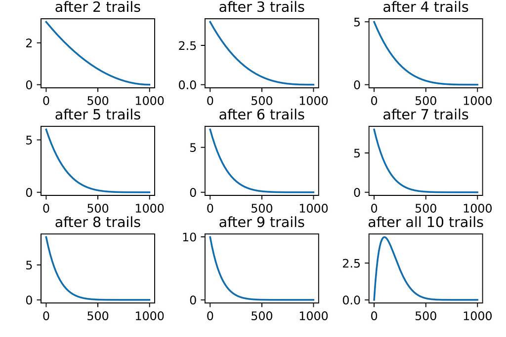
Assuming observations as [T,T,T,T,T,T,T,T,T,H]

#Lets import required packages
import numpy as np 
import matplotlib.pyplot as plt

#Taking a grid of 1000 points between 0 and 1
probability_grid = np.linspace(0,1,num= 1000)

#As we have assumed a uniform distribution between 0 and 1 (i.e. uniform distribution across all 1000 grid points)
prior_probability = np.ones(1000)

#Now lets toss the coin once, and we observed a tail
probability_data = binom.cdf(k=0, n=1, p=probability_grid)
posterior = prior_probability * probability_data 
posterior = (posterior/sum(posterior))*1000

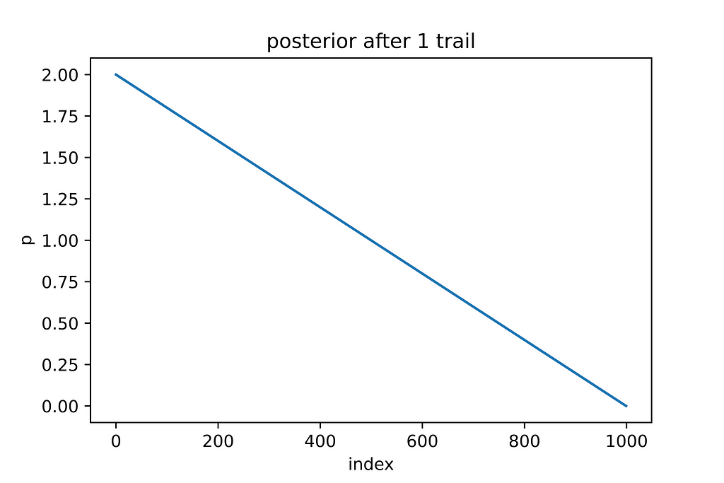
This process of posterior updating has to be repeated for all ten trails, and the posterior after each trail is shown below:

I iterated through all of the trails separately to demonstrate the procedure. We can use the Pymc3 package to do it in a single shot.

#Import required packages
import pymc3 as pm
import arviz as az
tosses_output = [ 0,0,0,0,0,0,0,0,0,1]

with pm.Model() as model:
    # lets define the prior
    hypo = pm.Beta('hypo', 2, 2)
    
    # define probability
    data = pm.Bernoulli('data', hypo, observed=tosses)
    
    # sample
    trace = pm.sample(return_inferencedata=True)

# visualize
az.plot_posterior(trace, hdi_prob=0.95)

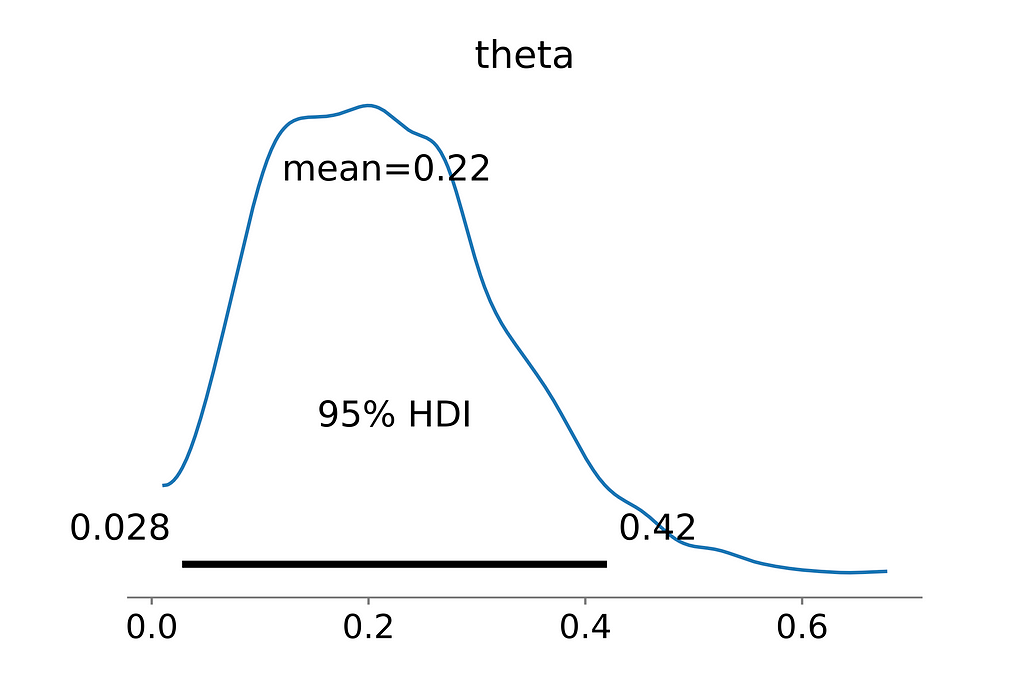
So, what did we accomplish? Rather than simply stating whether or not the coin is biased, we obtained the entire distribution of success, from which we can answer questions like the most likely probabilities of heads, Confidence Intervals of heads.

I’ll conclude with a cartoon to help you remember the distinction between Bayesian and frequentist thinking.

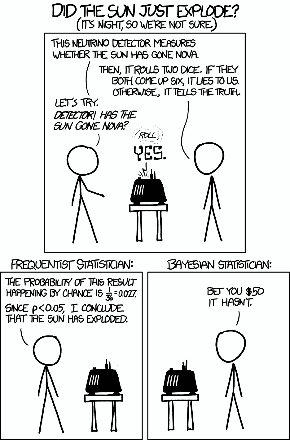
Frequentist inference does not account for the ‘prior’ probability of the sun exploding, and because it is based solely on observed data, a purely Frequentist method can run into problems. The Frequentist examines how likely the finding is in light of the null hypothesis, but it does not consider if the hypothesis is even more implausible a priori.

References and additional reading

[1] Frequentist and Bayesian Approaches in Statistics

[2] Comparison of frequentist and Bayesian inference

[3] The Signal and the Noise

[4] Bayesian vs Frequentist Approach

[5] Probability concepts explained: Bayesian inference for parameter estimation.

[6] Andre Schumacher’s talk at DTC

[7] Richard McElreath’s Statistical Rethinking lectures 2019

---

Bayesian Inference in Python was originally published in Towards AI on Medium, where people are continuing the conversation by highlighting and responding to this story.

Join thousands of data leaders on the AI newsletter. It’s free, we don’t spam, and we never share your email address. Keep up to date with the latest work in AI. From research to projects and ideas. If you are building an AI startup, an AI-related product, or a service, we invite you to consider becoming a sponsor.

Published via Towards AI