Analysis on the Biodiversity in National Parks Projects

Author(s): Karthik Bhandary

Originally published on Towards AI the World’s Leading AI and Technology News and Media Company. If you are building an AI-related product or service, we invite you to consider becoming an AI sponsor. At Towards AI, we help scale AI and technology startups. Let us help you unleash your technology to the masses.

Data Analysis

Analysis on Biodiversity in National Parks Projects

In this blog, we are going to be performing an analysis on the data set “Biodiversity in National Parks Projects”, which is available in Kaggle. We are going to be using visualizations and statistics to perform the analysis. Remember this is a simple analysis. We are not going to be applying any ML algorithms.

You can check out my notebook in Kaggle. If you like it, don’t forget to upvote it. With that said. let’s get into analysing the dataset.

Introduction

The goal of this project is to analyze biodiversity data from the National Parks Service, particularly around various species observed in different national park locations.

This project will scope, analyze, prepare, plot data, and seek to explain the findings from the analysis.

Here are a few questions that this project has sought to answer:

• What is the distribution of conservation status for species?
• Are certain types of species more likely to be endangered?
• Are the differences between species and their conservation status significant?
• Which animal is most prevalent and what is their distribution amongst parks?

Project Goals

In this project, the perspective will be through a biodiversity analyst for the National Parks Service. The National Park Service wants to ensure the survival of at-risk species, to maintain the level of biodiversity within their parks. Therefore, the main objectives as an analyst will be understanding the characteristics of the species and their conservations status, and those species and their relationship to the national parks. Some questions that are posed:

• What is the distribution of conservation status for species?
• Are certain types of species more likely to be endangered?
• Are the differences between species and their conservation status significant?
• Which animal is most prevalent and what is their distribution amongst parks?

Data

This project has two data sets that came with the package. The first csv file has information about each species and another has observations of species with park locations. This data will be used to analyze the goals of the project.

Analysis

In this section, descriptive statistics and data visualization techniques will be employed to understand the data better. The statistical inference will also be used to test if the observed values are statistically significant. Some of the key metrics that will be computed include:

1. Distributions
2. counts
3. relationship between species
4. conservation status of species
5. observations of species in parks.

Evaluation

Lastly, it’s a good idea to revisit the goals and check if the output of the analysis corresponds to the questions first set to be answered (in the goals section). This section will also reflect on what has been learned through the process, and if any of the questions were unable to be answered. This could also include limitations or if any of the analysis could have been done using different methodologies.

Importing Necessary Modules

import pandas as pd
import numpy as np
import matplotlib.pyplot as plt
import seaborn as sns
%matplotlib inline

Loading The Data

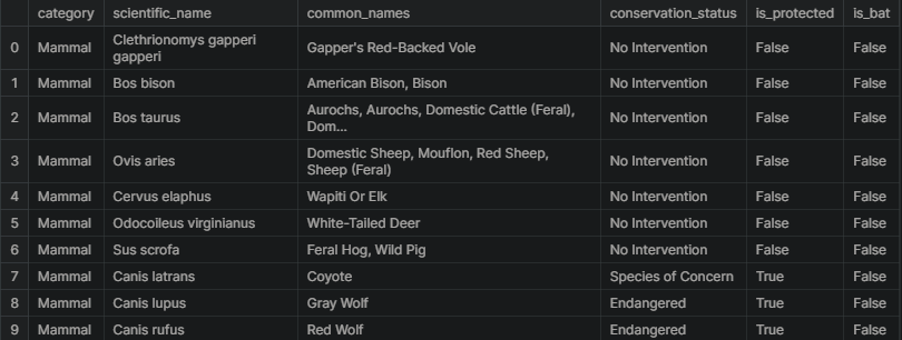
In the next steps, Observations.csv and Species_info.csv are read in as DataFrames called observations and species respectively. The newly created DataFrames are glimpsed with .head() to check its contents.

species = pd.read_csv("../input/biodiversity-in-national-parks-project/species_info.csv")
species.head()

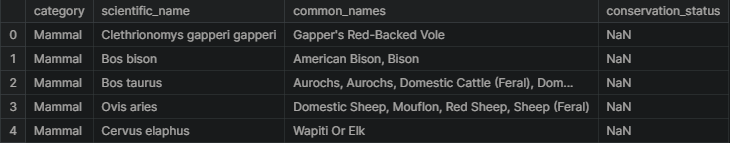
It loads the following result

observations = pd.read_csv("../input/biodiversity-in-national-parks-project/observations.csv")
observations.head()

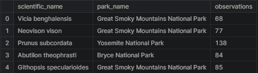
We get the following result

Data Characteristics

Next, there will be a check for the dimensions of the data sets, for species there are 5,824 rows and 4 columns while observations has 23,296 rows and 3 columns.

print(f"Species Shape: {species.shape}")
print(f"Observations Shape: {observations.shape}")

#Result
Species Shape: (5824, 4)
Observations Shape: (23296, 3)

It is time to explore the species data a little more in-depth. The first thing is to find the number of distinct species in the data.

print(f"No of unique species: {species.scientific_name.nunique()}")

#Result
No of unique species: 5541

print(f"No of unique categories: {species.category.nunique()}")
print(f"Categories: {species.category.unique()}")

#Result
No of unique categories: 7
Categories: ['Mammal' 'Bird' 'Reptile' 'Amphibian' 'Fish' 'Vascular Plant'
 'Nonvascular Plant']

species.groupby("category").size()

#Result
category
Amphibian              80
Bird                  521
Fish                  127
Mammal                214
Nonvascular Plant     333
Reptile                79
Vascular Plant       4470
dtype: int64

From the above observations made, Vascular plants are by far the largest share of species with 4,470 in the data with reptiles being the fewest with 79.

print(f"No of unique status: {species.conservation_status.nunique()}")
print(f"Conservation Status: {species.conservation_status.unique()}")

#Result
No of unique status: 4
Conservation Status: [nan 'Species of Concern' 'Endangered' 'Threatened' 'In Recovery']

Next, a count of the number of observations in the breakdown of the categories in conservation_status is done. There are 5,633 nan values which means that they are species without concerns. On the other hand, there are 161 species of concern, 16 endangered, 10 threatened, and 4 in recovery.

print(f"na Values: {species.conservation_status.isna().sum()}")
print(species.groupby('conservation_status').size())

#Result
na Values: 5633
conservation_status
Endangered             16
In Recovery             4
Species of Concern    161
Threatened             10
dtype: int64

observations

The next section looks at the observations data. The first task is to check the number of parks that are in the dataset and there are only 4 national parks.

print(f"No. of Parks: {observations.park_name.nunique()}")
print(f"Parks: {observations.park_name.unique()}")

#Result
No. of Parks: 4
Parks: ['Great Smoky Mountains National Park' 'Yosemite National Park'
 'Bryce National Park' 'Yellowstone National Park']

Here are the total number of observations logged in the parks, there are 3,314,739 sightings in the last 7 days… that’s a lot of observations!

print(f"observations: {observations.observations.sum()}")

#Result
observations: 3314739

Analysis

The first task will be to clean and explore the conservation_status column in species.

The column conservation_status has several possible values:

• Species of Concern: declining or appear to require conservation
• Threatened: vulnerable to endangerment soon
• Endangered: seriously at risk of extinction
• In Recovery: formerly Endangered, but currently neither in danger of extinction throughout all or a significant portion of its range

In the exploration, a lot of nan values were detected. These values will need to be converted to No Intervention.

species.conservation_status.fillna("No Intervention", inplace=True)
species.groupby("conservation_status").size()

#Result

conservation_status
Endangered              16
In Recovery              4
No Intervention       5633
Species of Concern     161
Threatened              10
dtype: int64

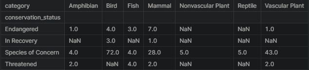
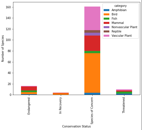
Next is to check out the different categories that are nested in the conservation_status column except for the ones that do not require an intervention. There is both the table and chart to explore below.

For those in the Endangered status, 7 were mammals and 4 were birds. In the In Recovery status, there were 3 birds and 1 mammal, which could mean that the birds are bouncing back more than the mammals.

conservationCategory = species[species.conservation_status != 'No Intervention']\
.groupby(["conservation_status", "category"])["scientific_name"]\
.count()\
.unstack()
conservationCategory

ax = conservationCategory.plot(kind="bar", figsize=(8,6), stacked=True)
ax.set_xlabel("Conservation Status")
ax.set_ylabel("Number of Species");

In conservation

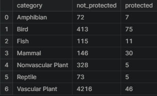
The next question is if certain types of species are more likely to be endangered? This can be answered by creating a new column called is_protected and include any species that had a value other than No Intervention.

species['is_protected'] = species.conservation_status != 'No Intervention'

category_counts = species.groupby(['category', 'is_protected'])\
                        .scientific_name.nunique()\
                        .reset_index()\
                        .pivot(columns='is_protected',
                                      index='category',
                                      values='scientific_name')\
                        .reset_index()
category_counts.columns = ['category', 'not_protected', 'protected']

category_counts

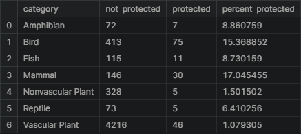
category_counts['percent_protected'] = category_counts.protected / \
                                      (category_counts.protected + category_counts.not_protected) * 100

category_counts

Statistical Significance

This section will run some chi-squared tests to see if different species have statistically significant differences in conservation status rates. To run a chi-squared test, a contingency table will need to be created. The contingency table should look like this:

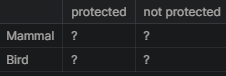
The first test will be called contingency1 and will need to be filled with the correct numbers for mammals and birds.

The results from the chi-squared test returns many values, the second value which is 0.69 is the p-value. The standard p-value to test statistical significance is 0.05. For the value retrieved from this test, the value of 0.69 is much larger than 0.05. In the case of mammals and birds, there doesn’t seem to be any significant relationship between them i.e. the variables independent.

from scipy.stats import chi2_contingency

contingency1 = [[30, 146],
              [75, 413]]
chi2_contingency(contingency1)

#Result

(0.1617014831654557,
 0.6875948096661336,
 1,
 array([[ 27.8313253, 148.1686747],
        [ 77.1686747, 410.8313253]]))

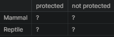
The next pair is going to test the difference between Reptile and Mammal.

The format is again is like below:

This time the p-value is 0.039 which is below the standard threshold of 0.05 which can be taken that the difference between reptile and mammal is statistically significant. Mammals are shown to have a statistically significant higher rate of needed protection compared with Reptiles.

contingency2 = [[30, 146],
               [5, 73]]
chi2_contingency(contingency2)

#Result

(4.289183096203645,
 0.03835559022969898,
 1,
 array([[ 24.2519685, 151.7480315],
        [ 10.7480315,  67.2519685]]))

species in parks

The next set of analyses will come from data from the conservationists as they have been recording sightings of different species at several national parks for the past 7 days.

The first step is to look at the common names species to get an idea of the most prevalent animals in the dataset. The data will need to be split up into individual names.

from itertools import chain
import string

def remove_punctuations(text):
    for punctuation in string.punctuation:
        text = text.replace(punctuation, '')
    return text

common_Names = species[species.category == "Mammal"]\
    .common_names\
    .apply(remove_punctuations)\
    .str.split().tolist()

common_Names[:6]

#Result

[['Gappers', 'RedBacked', 'Vole'],
 ['American', 'Bison', 'Bison'],
 ['Aurochs',
  'Aurochs',
  'Domestic',
  'Cattle',
  'Feral',
  'Domesticated',
  'Cattle'],
 ['Domestic', 'Sheep', 'Mouflon', 'Red', 'Sheep', 'Sheep', 'Feral'],
 ['Wapiti', 'Or', 'Elk'],
 ['WhiteTailed', 'Deer']]

The next step is to clean up duplicate words in each row since they should not be counted more than once per species.

cleanRows = []

for item in common_Names:
    item = list(dict.fromkeys(item))
    cleanRows.append(item)
    
cleanRows[:6]

#Result

[['Gappers', 'RedBacked', 'Vole'],
 ['American', 'Bison'],
 ['Aurochs', 'Domestic', 'Cattle', 'Feral', 'Domesticated'],
 ['Domestic', 'Sheep', 'Mouflon', 'Red', 'Feral'],
 ['Wapiti', 'Or', 'Elk'],
 ['WhiteTailed', 'Deer']]

res = list(chain.from_iterable(i if isinstance(i, list) else [i] for i in cleanRows))
res[:6]

#Result

['Gappers', 'RedBacked', 'Vole', 'American', 'Bison', 'Aurochs']

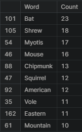
Now the data is ready to be able to count the number of occurrences of each word. From this analysis, it seems that Bat occurred 23 times while Shrew came up 18 times.

words_counted = []

for i in res:
    x = res.count(i)
    words_counted.append((i,x))

pd.DataFrame(set(words_counted), columns =['Word', 'Count']).sort_values("Count", ascending = False).head(10)

In the data, there are several different scientific names for different types of bats. The next task is to figure out which rows of species are referring to bats. A new column made up of boolean values will be created to check if is_bat is True.

species['is_bat'] = species.common_names.str.contains(r"\bBat\b", regex = True)

species.head(10)

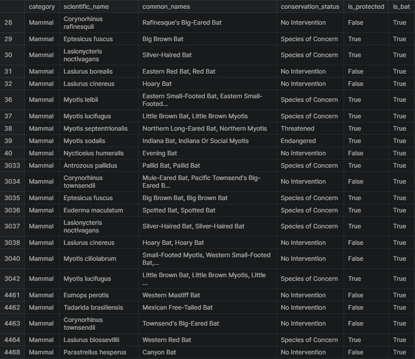
Here is a subset of the data where is_bat is true, returning see the rows that matched. There seems to be a lot of species of bats and a mix of protected vs. non-protected species.

species[species.is_bat]

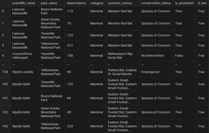
Next, the results of the bat species will be merged with observations to create a DataFrame with observations of bats across the four national parks.

bat_observations = observations.merge(species[species.is_bat])
bat_observations

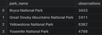
Let’s see how many total bat observations(across all species) were made at each national park.

The total number of bats observed in each park over the past 7 days are in the table below. Yellowstone National Park seems to have the largest with 8,362 observations and the Great Smoky Mountains National Park has the lowest with 2,411.

bat_observations.groupby('park_name').observations.sum().reset_index()

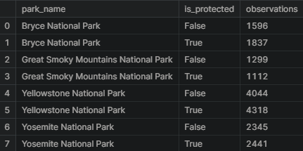
Now let’s see each park broken down by protected bats vs. non-protected bat sightings. It seems that every park except for the Great Smoky Mountains National Park has more sightings of protected bats than not. This could be considered a great sign for bats.

obs_by_park = bat_observations.groupby(['park_name', 'is_protected']).observations.sum().reset_index()
obs_by_park

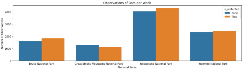
Below is a plot from the output of the last data manipulation. From this chart, one can see that Yellowstone and Bryce National Parks seem to be doing a great job with their bat populations since there are more sightings of protected bats compared to non-protected species. The Great Smoky Mountains National Park might need to beef up their efforts in conservation as they have seen more non-protected species.

plt.figure(figsize=(16, 4))
sns.barplot(x=obs_by_park.park_name, y= obs_by_park.observations, hue=obs_by_park.is_protected)
plt.xlabel('National Parks')
plt.ylabel('Number of Observations')
plt.title('Observations of Bats per Week')
plt.show()

Conclusions

The project was able to make several data visualizations and inferences about the various species in four of the National Parks that comprised this data set.

This project was also able to answer some of the questions first posed in the beginning:

1. What is the distribution of conservation status for species?

• The vast majority of species were not part of conservation. (5,633 vs 191)

2. Are certain types of species more likely to be endangered?

• Mammals and Birds had the highest percentage of being in protection.

3. Are the differences between species and their conservation status significant?

• While mammals and birds did not have significant differences in conservation percentage, mammals and reptiles exhibited a statistically significant difference.

3. Which animal is most prevalent and what is their distribution amongst parks?

• the study found that bats occurred the most number of times and they were most likely to be found in Yellowstone National Park.

I really hope that you found this analysis helpful and interesting. If you liked my work then don’t forget to follow me on Medium and YouTube, for more content on productivity, self-improvement, Coding, and Tech. Also, check out my works on Kaggle and follow me on LinkedIn.

Check out my recent works:

• Basic SQL for DataScience Part-1
• Joins with Pandas Dataframes

---

Analysis on the Biodiversity in National Parks Projects was originally published in Towards AI on Medium, where people are continuing the conversation by highlighting and responding to this story.

Join thousands of data leaders on the AI newsletter. It’s free, we don’t spam, and we never share your email address. Keep up to date with the latest work in AI. From research to projects and ideas. If you are building an AI startup, an AI-related product, or a service, we invite you to consider becoming a sponsor.

Published via Towards AI