AI at Rescue: Demand Forecasting

Author(s): Supreet Kaur

Originally published on Towards AI the World’s Leading AI and Technology News and Media Company. If you are building an AI-related product or service, we invite you to consider becoming an AI sponsor. At Towards AI, we help scale AI and technology startups. Let us help you unleash your technology to the masses.

Demand Forecasting is a field of predictive analytics that predicts customer demand based on historical data and other related variables to drive the supply chain decision-making process.

Machine Learning models can come to your rescue to predict accurate demand. Many models are available for your disposal, but it is essential to tailor the model as per the industry and data in hand.

This blog is an end-to-end guide on leveraging AI to perform demand forecasting, including preparing your data, choosing the models, and measuring their accuracy.

Impact of accurate Demand Forecasting

1. Minimize wastage of products
2. Reduce Inventory Costs
3. Assists in planning the production of a product
4. Enhancing customer experience by providing the product exactly when it is needed

Preparing your Data

All of us are aware of the concept “Garbage In, Garbage Out.” Hence it is inevitable to prepare your data so that it is ready to be ingested by the ML or statistical models.

Here are a few primary attributes you would require in your dataset to perform demand forecasting:

1. Unique ID(Customer/Patient)
2. Product Name
3. A number of units sold.

Note: This can vary from industry to industry. You must ensure that the scale is consistent in the dataset. Example: It could be the SKU of a particular product

4. Timestamp

Once you have the dataset, it is crucial to observe a few things before you proceed to your ML models:

1. Trend: A trend is observed to gauge whether it is an increasing or decreasing demand. Suppose you observe some unexplained highs or lows. In that case, it is crucial to analyze those outliers before performing any model, as it can create unnecessary bias in your dataset.
2. Seasonality: Seasonality is influenced by a specific time of the year. For example, retail companies observe a spike in sales during the holiday season, which is cyclic, i.e., it repeats every year at the same time. An important thing to note here is that a few events like COVID influenced the sales as people hoarded, but that was one of a kind, so we can’t consider it a seasonal pattern.
3. Noise: This is a common observation in time-series datasets. You might observe a particular trend, but at the same time, you might see a few random points(outliers) that any business justification cannot explain.

Machine Learning Models

The golden rule to building any AI-driven solution is to start with vanilla models and analyze if it is a good fit for your data. This section will cover both vanilla and advanced ML algorithms:

1. ARIMA

The ARIMA is a statistical technique to forecast time series data. It stands for Autoregressive Integrated Moving Average. Any machine learning model is autoregressive if it predicts future values based on past weights. Let’s break it down further:

1. AR(Autoregression): represents the use of previous data to predict the next value
2. I(Integrated): subtracting a given value with the previous value to make the time series stationary
3. MA(Moving Average): leveraging the error terms themselves to predict future values

The parameter of ARIMA is as follows and should be chosen wisely based on your data:

1. P: Number of lag observations(previous data) in the model

2. D: Number of times raw observations are differenced

3. Q: Order of Moving Average

In R or python, you can use Auto-Arima to specify a range for the above hyperparameters, and it will choose the best one catering to your dataset on AIC and BIC values.

Advantages

1. Easy to interpret
2. Ideal for short-term forecasts

Limitations

1. Poor performance in case of long-term forecasts
2. It can’t be leveraged for seasonal time series

2. HOLT-WINTER’S METHOD

Holt Winter’s method is called triple exponential smoothing as the three components of time series behavior, such as value(average), trend(slope), and seasonality, are expressed as three types of exponential smoothing. The model outputs the forecast by computing the combined effort of these three influences.

The parameters required for this model are:

1. (ɑ, β, γ) one for each smoothing
2. The length of a season
3. The number of periods in a season

The smoothing is applied across seasons, e.g., the seasonal component of the 3rd point into the season would be exponentially smoothed with the one from the 3rd point of last season, the 3rd point two seasons ago, etc. In math notation, we now have four equations (see footnote):

ℓx=α(yx−sx−L)+(1−α)(ℓx−1+bx−1)

bx=β(ℓx−ℓx−1)+(1−β)bx−1

sx=γ(yx−ℓx)+(1−γ)sx−L

y^x+m=ℓx+mbx+sx−L+1+(m−1)modL

Holt’s winter’s method is an extension of exponentially weighted moving average methods (EWMA). The EWMA is not suitable for time series with a linear trend. Holt-Winters method uses exponential smoothing to encode values from the past and then use them to predict typical values from the future.

Advantages

1. Provides accurate prediction on actual-world data as it considers seasonality and trend, which is inevitable in correct world data

Limitations

1. The model might not be the best fit when we have time frames with meager amounts, such as a time frame with a data point of 10 or 1 might have an actual difference of 9, but there is a relative difference of about 1000%.

3. PROPHET by Facebook

The prophet is a library in R and Python equipped to forecast time series. It is mighty to capture change points such as the rise and fall of COVID cases. You also have the flexibility to control the power of these changepoints.

The parameters include:

1. growth: choose between ‘linear’ or ‘logistic’ trend
2. changepoints: List of dates accommodating potential changepoints (automatic if not specified)
3. n_changepoints: If changepoints are not supplied, provide the number of changepoints to be automatically included
4. changepoint_prior_scale: Parameter for changing flexibility of automatic changepoint selection

Advantages

1. Flexibility to control uncertainty, trend, changepoint, and holiday effect
2. Easy to interpret and use even for people with little or no knowledge of data science/forecasting

Limitations

1. Low Accuracy
2. Unable to detect causal relationships between the past and future data
3. Lacks the ability to forecast data with weak seasonality

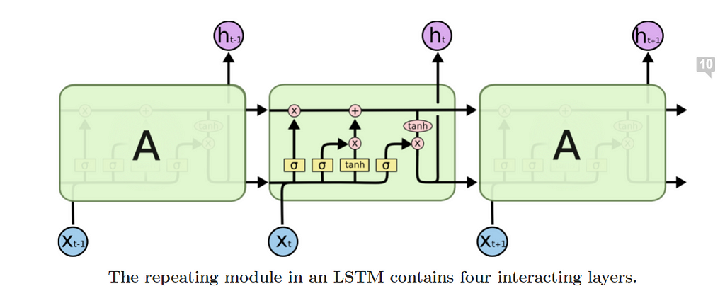
4. LSTM’s

Long Short-Term Memory RNN’s are known for learning long-term sequences. It does not depend on pre-specified window lagged observation as input. RNNs suffer the loss of information due to vanishing gradient problems. Still, LSTMs don’t suffer from this issue as recurrent weights array is replaced by identity function and controlled by a series of gates such as input, output, and forget gate.

Few data preparation steps are needed to pursue before prepping this model:

· Make the dataset stationary: You can do this by simple techniques like differencing.

· Transform the data as per the scale of the activation function

Advantages

· Higher accuracy

Validating your Model/ Measuring Accuracy

You can use different calculations to measure the accuracy of your model depending on the industry and data. Some of the standard measures are as follows:

1. MAPE

MAPE (Mean Absolute Percentage Error) measures the size of the error in percentage terms. The MAPE should not be used with low-volume data as it will take on extreme values.

(1/n∑|Actual-Forecast|/|Actual|) *100

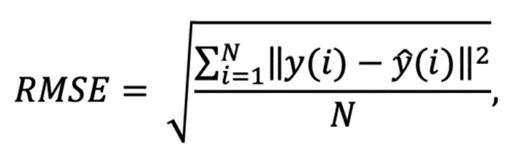
2. RMSE

Root Mean Squared Error is one of the most used measures to evaluate the quality of predictions. It shows how far predictions fall off when measured from actual values using Euclidean distance. This is a good measure for LSTM forecasts.

N is the number of data points, y(i) is the ith measurement, and y ̂(i) is its corresponding prediction.

N is the number of data points, y(i) is the ith measurement, and y ̂(i) is its corresponding prediction

Happy Reading!

References:

https://machinelearningmastery.com/arima-for-time-series-forecasting-with-python/

https://www.analyticsvidhya.com/blog/2021/07/abc-of-time-series-forecasting/

https://www.rdocumentation.org/packages/forecast/versions/8.16/topics/auto.arima

https://grisha.org/blog/2016/02/17/triple-exponential-smoothing-forecasting-part-iii/

https://www.capitalone.com/tech/machine-learning/understanding-arima-models/

https://medium.com/swlh/facebook-prophet-426421f7e331

https://analyticsindiamag.com/why-are-people-bashing-facebook-prophet/

https://machinelearningmastery.com/time-series-forecasting-long-short-term-memory-network-python/

How do I measure forecast accuracy?

https://www.analyticsvidhya.com/blog/2018/05/generate-accurate-forecasts-facebook-prophet-python-r/

---

AI at Rescue: Demand Forecasting was originally published in Towards AI on Medium, where people are continuing the conversation by highlighting and responding to this story.

Join thousands of data leaders on the AI newsletter. It’s free, we don’t spam, and we never share your email address. Keep up to date with the latest work in AI. From research to projects and ideas. If you are building an AI startup, an AI-related product, or a service, we invite you to consider becoming a sponsor.

Published via Towards AI