A Surefire Way to Building a Neural Network Using Python

Author(s): Abhishek Kumar

Originally published on Towards AI.

Do you ever wonder how the browse feeds of your Netflix, YouTube, or Instagram Accounts can be so riveting so as to kill hours of your time against your will? Or how there are apps like Youper or Moodpath carrying out therapies for anxiety and depression? The answer to all of those questions that make you wonder that there is a brain inside your gadget when there are just silicon chips in there is neural networks.

Let’s get a hold of what they are and their basic skeletons. To do this, we will be using Python as the primary language because of its obvious benefits.

What is a Neural Network?

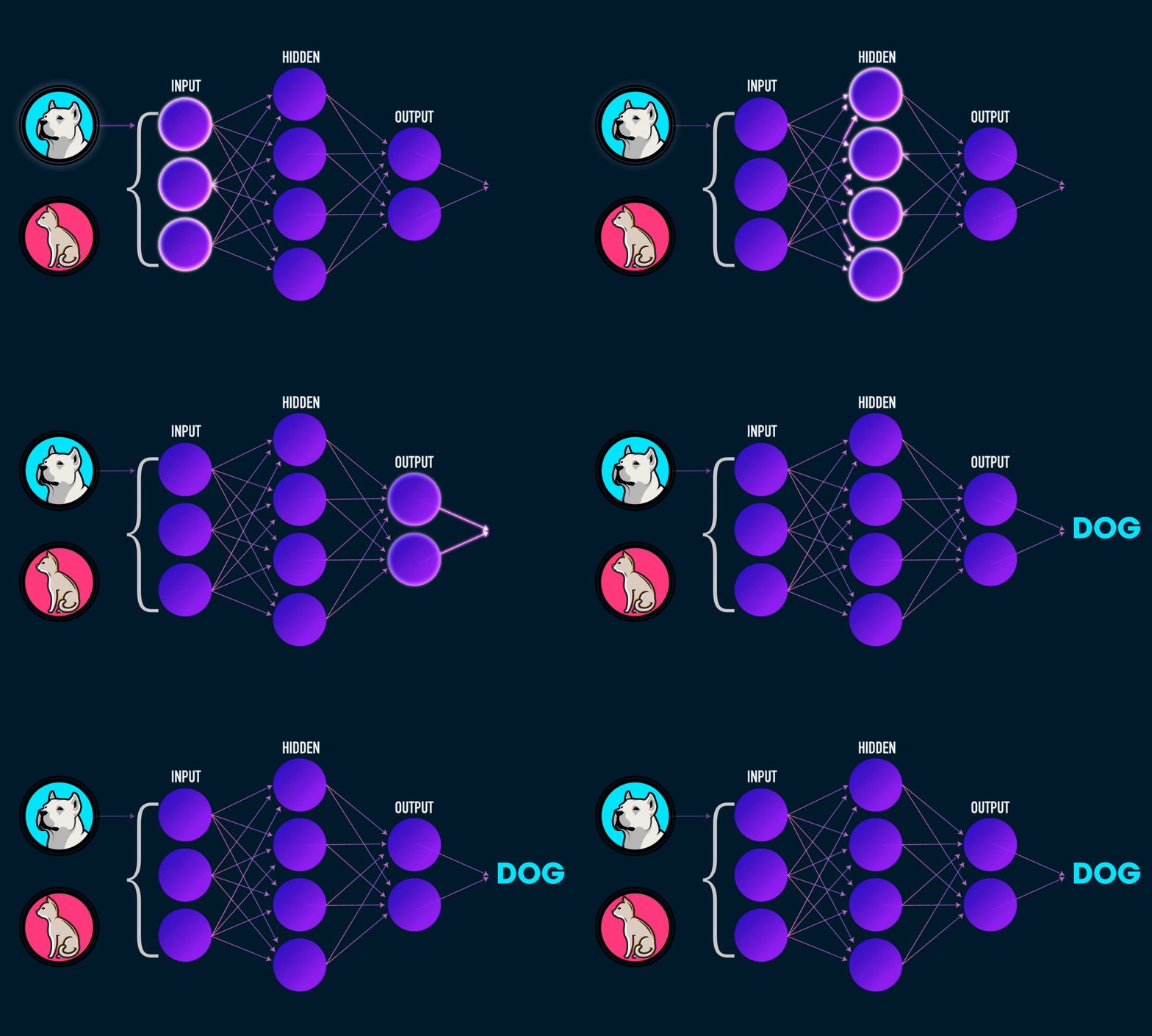
Whenever someone starts to explain about neural networks, they always seem to keep a human brain as a premise. But I feel that any system that gives an output for a provided input can be deemed analogous to a neural network. That is what a neural network is, a mathematical function with a layer of inputs comprised of independent variables, multiple arbitrary hidden layers, an activation function culled from all the choices for each hidden layer, their respective weights, and biases, and finally a layer of outputs containing dependent variables.

After you’ve created the framework of the neural network, you have to train it. Now, a system’s core network is not the most imperative part of the system because it might give out the output, but it doesn’t answer questions about the output’s credibility. Hence comes a need for a sub-network in all neural networks that can identify the error i.e., the difference between actual values or the desired output and the propagated values. The sub-network that determines the error is called the cost network or the cost function. At first, the neural network predicts some random values, and cost or error is calculated. Theron, we aim to attenuate the cost and imbricate the actual and propagated values.

For a topic like this, it would be straightforward obfuscation not to introduce an example. Let us take an example in which the inputs are age, smoking, area of residence, and genetic health history with their respective weights and output is the chance of having a lung disease. All of the input nodes are denoted by x for generality. W denotes the weight carried by each input node, which might keep changing as the execution proceeds. The respective biases of each step are denoted by b.

Implementation By Neural Networks

To execute a task, a neural network has to go through two steps that are explained below:

Feed Forward

The predictions made by a neural network based on the values of inputs and their respective weights are made by the feed-forward network of the neural network. You might see four features in the dataset: age, smoking, area of residence, and genetic health history.

The weights in a neural network are basically strings that we tune by taking into account the error feedback so as to predict the output accurately. You must keep one thing at the core right now that for each input node, there is a weight.

The first step to execute the feed-forward phase is to calculate the dot products of the values provided by the input layers and their respective weight parameters. Then dot products of all the nodes are summed together and added with a bias term b. It promises a robust neural network by providing an output even if all the input nodes carry a zero value. For instance, if there is a young person who doesn’t smoke, lives in an area with minimal pollutants, and has no genetic history of lung diseases, the outputs are almost going to be zero. So we introduce a bias term, which will be corrected accordingly as we provide supporting data.

????.????= ????1????1+????2????2+????3????3+????4????4+b

This step can yield any set of values. But we need to align these values derived from the input with the values that can be yielded by the output i.e., 0 or 1. Here the activation function kicks in, here taken as the sigmoid function. It helps us squashing these values between 0 and 1.

If we try entering the value zero, the function returns 0.5 as output. It returns a value of 1 if the input is a large positive number. Clearly, for all the sets of values propagated by the first step, the input is going to be between 0 and 1. We can also check this by plotting the sigmoid function.

We use NumPy Library and matplotlib library for doing so. We generate 200 linearly spaced points between -10 and 10 using the linspace method and assign it to the variable ‘input’ from the NumPy library. We then define the sigmoid function and plot sigmoid vs. input using the matplotlib library.

The output for this script comes as:

It is evident that even if the input nodes produce negative values after the first step, the sigmoid function helps us to make the values between 0 and 1.

This wraps up the feed-forward phase of the neural networks. First, we find the dot product of the matrices of input nodes by their respective weight matrix with a bias for a rigorous network. Then we pass these values through the activation function, and then we have a set of values that are to be called the ‘propagated values.’

Backpropagation

When the neural network first executes a task without any training, it makes random predictions that need a precision wand to be waved. This precision is achieved by the process of backpropagation. Once the predictions are made, we then compare those predicted values with the actual output. Then the computed error is used to tune the weights and biases in order to establish concordance between the yielded output and actual output. This process of backpropagation is also known as “Training the algorithm.” This is perhaps the part that makes Python really special for AI/ML projects.

To train the algorithm, we first need to calculate the cost or loss of the predicted values. Higher the difference between the actual and predicted output higher the loss is. We need a loss function to execute this. We use the Mean Squared Error as our loss function out of the myriad choices for the loss function.

Once we have calculated the cost using the cost function, we then aim to minimize it by tweaking the choice of our weights and biases. So this step of the backpropagation phase is nothing but an optimization problem where we need to find the function minima. We can hence use many optimization techniques to find the minimum cost and by finding the variance in cost with varying weights and biases and set their values accordingly.

Wrapping Up:

In this article, the underlying framework of a basic neural network has been discussed. Although there are a plethora of deep learning libraries that can be used to bring neural networks to life in a few lines of code, it is always good to have a grasp on the basics. Hereon, you can see for yourself the different changes to be made in a neural network, when you are designing a recommender system for a digital content platform or a chatbot giving freemium therapy to teenagers.

Join thousands of data leaders on the AI newsletter. Join over 80,000 subscribers and keep up to date with the latest developments in AI. From research to projects and ideas. If you are building an AI startup, an AI-related product, or a service, we invite you to consider becoming a sponsor.

Published via Towards AI