A Short Journey To Deep Learning

Author(s): Bala Gopal Reddy Peddireddy

Originally published on Towards AI the World’s Leading AI and Technology News and Media Company. If you are building an AI-related product or service, we invite you to consider becoming an AI sponsor. At Towards AI, we help scale AI and technology startups. Let us help you unleash your technology to the masses.

Understanding Artificial Neural Network (ANN) With An Example…🫀

Overview of the article

This article is mainly about the understanding of Artificial neural networks (ANN) and their workflow. When you listen to these words, you might have many questions like:

What is Deep Learning?

How does the Biological and Artificial Neuron work?

What is a Perceptron (ANN)?

How does a deep learning model get trained?

All these questions are addressed in the article. A detailed explanation of the example is included in the article that has steps like:

Description of the dataset

Import the packages and Dataset

Exploratory Data Analysis

Data Pre-Processing

Create, Train, Predict, and Evaluate an ANN model

Let’s Get Started

What is Deep Learning?

Deep learning is a part of Machine Learning that mainly focuses on Artificial Neural Networks that would try to mimic the brain. Deep learning was introduced in the early 50s but it became popular in recent years due to the increase in AI-oriented applications and the data that is being generated by the companies.

In my view, It is easy to understand the concepts individually but when you implement them together it would be difficult to follow what’s going on inside the model. That’s why deep learning models are often called the black-box model. However, It would give amazing results to our business problem and it has a lot of applications.

How does the Biological and Artificial Neuron work?

Let me explain a scenario when you touch a hot object with your hand, you would feel the pain and remove the hand immediately. This action and reaction are done within a fraction of a second. Have you ever got a feeling that how this is happening?

Well, they are trillions of neurons connected in the body when you touch a hot object the electrical impulse will travel from the neurons in your hand to the neurons in your brain. Then the decision is taken and immediately electrical impulse travels back to the neurons in hand instructing to remove it.

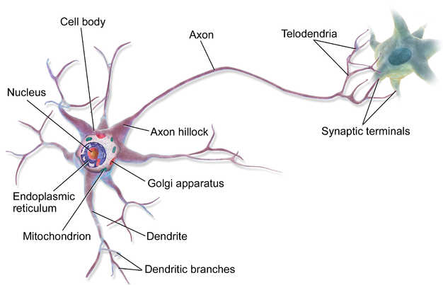
Inside neurons, Dendrites act as neuro receptors nothing but the input layer. Axons act as neurotransmitters nothing but the output layer. The nucleus is where the action potential is compared to the threshold. If the action potential is greater than the threshold, the electrical impulse will transmit to another neuron. If the action potential is lesser than the threshold, the electrical impulse won’t transmit to another neuron.

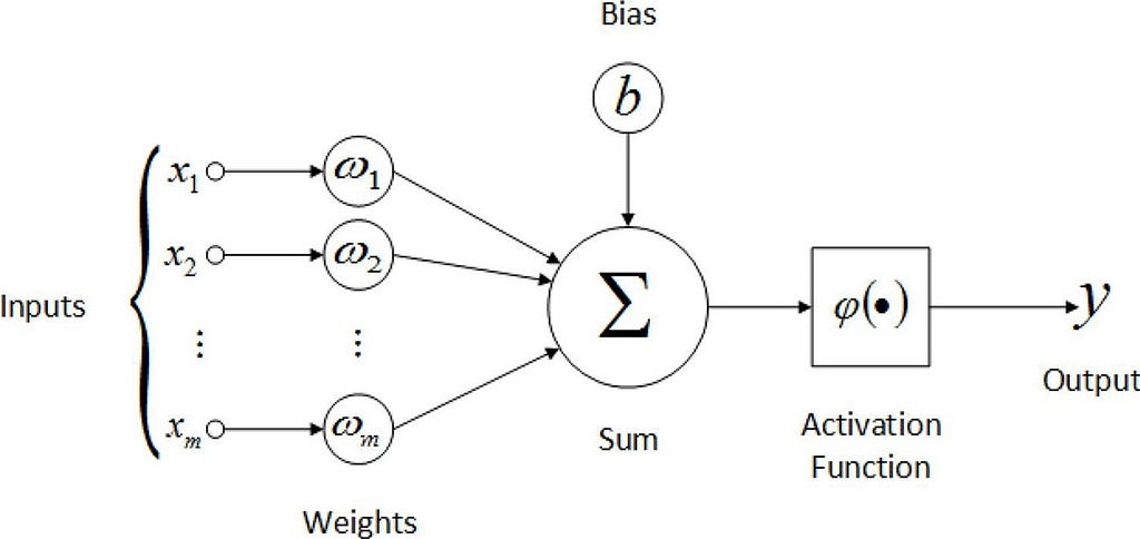
Similarly, artificial neurons receive the information from the input layer and transmit the information to other neurons through the output layer. Here, the neurons are connected and certain weights are assigned to that particular connection. These weights represent the strength of the connection and they play an important role in the activation of the neuron. The bias is like an intercept in the linear equation.

Here, the inputs (x1 to xn) get multiplied with corresponding weights (w1 to wn) and then they get summated along with the bias. The result would be taken as input for the activation function this is where the decision happens and the output of the activation function is transferred to other neurons. There are different types of activation functions some are linear, step, sigmoid, RelU, etc.

What is a Perceptron?

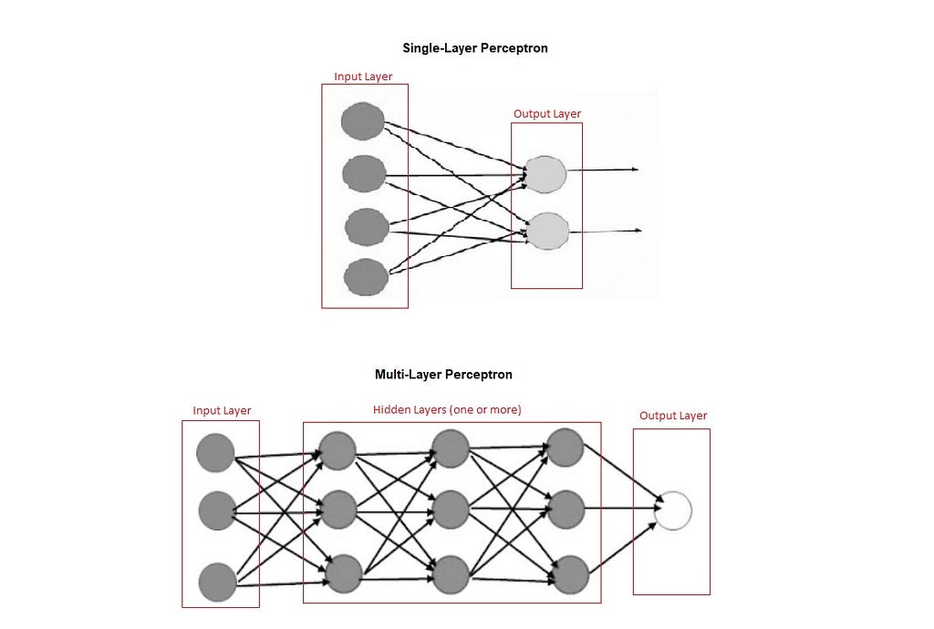
Perceptron is an algorithm that makes the neurons learn from the given information. It is of two types, Single-layer Perceptron does not contain hidden layers. Whereas, Multi-layer Perceptron contains one or more hidden layers. Single-layer Perceptron is the simplest form of an Artificial neural network (ANN).

How does a deep learning model get trained?

In forward propagation, the information goes from the input layer to the output layer. Here, the inputs get multiplied with corresponding weights then they get summated along with the bias, and then the activation function gets applied to that result. This process continues till it reaches the output layer with the predicted value(output). The loss function would find the error between the predicted and real output.

The whole idea of backward propagation is to decrease the error by updating the weights. This can be achieved with the help of optimizers. Here, the weights get updated from the last layer to the first layer by implementing the derivative rule. So, these both steps go on till you get the desired accuracy.

Example

Consider an example, Let’s work on the Heart Failure Prediction dataset. This is a classification problem, we will be predicting whether a patient has heart failure or not.

About the Dataset

The dataset contains 299 entries collected at the Faisalabad Institute of Cardiology in 2015. There are 105 females and 194 males in the age range between 40 and 95 years in the dataset. It contains 13 features that are:

• age: Patient’s age
• anemia: Whether the patient’s hemoglobin is below the normal range or not
• creatinine_phosphokinase: Creatine phosphokinase’s level in the blood (mcg/L)
• diabetes: Whether the patient was diabetic or not
• ejection_fraction: It is a measure of blood the left ventricle pumps out in each contraction.
• high_blood_pressure: Whether the patient has hypertension
• platelets: Count of the platelets in the blood (kiloplatelets/mL)
• serum_creatinine: Serum creatinine level in the blood (mg/dL)
• serum_sodium: Serum sodium level in the blood (mEq/L)
• sex: Gender of the patient
• smoking: Whether the patient smokes or not
• time: Patient’s follow-up visit time about the disease in months
• DEATH_EVENT: Whether the patient deceased due to heart failure

Import the packages

Firstly, import the required packages for exploring, visualizing, and preprocessing the data. These can be done with the help of pandas, Scipy, NumPy, matplolib, and seaborn libraries. Let’s import the warnings library as well to ignore the warning generated by the code.

Code:

import pandas as pd
import numpy as np
import scipy
import matplotlib.pyplot as plt
import seaborn as sns
%matplotlib inline
import warnings
warnings.filterwarnings('ignore')

Import the Dataset

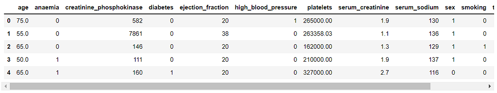
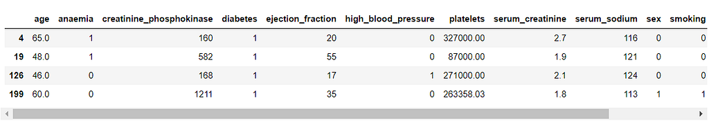
Import the dataset(heart_failure_clinical_records_dataset.csv)with the help of the read_csv method in the pandas package.

Code:

df=pd.read_csv('heart_failure_clinical_records_dataset.csv')
df.head()

Exploratory Data Analysis

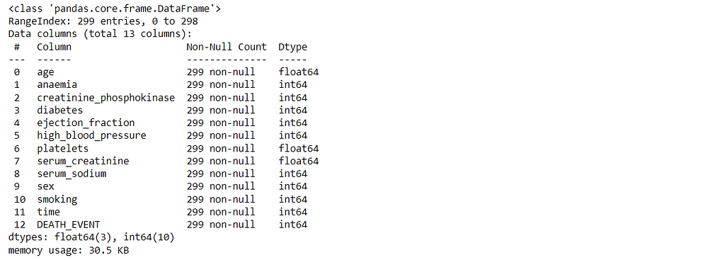
There are a lot of things to explore about the dataset. Let’s start with the description and information of the dataset with the help of the describe and info methods.

Code:

df.describe()

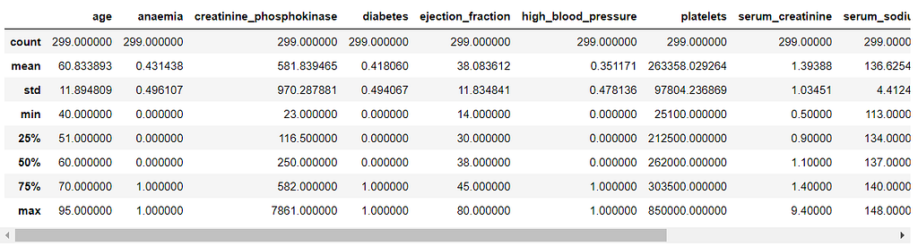
df.info()

Check for the Null values

It’s always important to check whether there are any null values in the dataset. If present, they must be handled because it might impact the model’s accuracy and you could get undesired results.

Code:

df.isnull().sum()

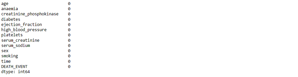
Luckily, The dataset does not contain any missing values. Otherwise, they needed to be handled with the help of the techniques like imputation, deletion, etc.

Data visualization

It is a way to analyze the data by visualizing the trends and patterns in the form of graphs, charts, plots, etc. They are different types of visualizations:

• Uni-variate analysis: Deals with one variable and find the pattern within the variable
• Bi-variate analysis: Deals with two variables and mainly focus on the relationship between them.
• Multi-variate analysis: Deals with more than two variables and checks the overall behavior of variables at the same time.

1. Let’s start the data visualization with the target variable to check the number of patients recovered and deceased by using the countplot method from the seaborn library.

Code:

plt.figure(figsize=(3,3),dpi=150)
sns.countplot(x="DEATH_EVENT", data=df,palette='rocket')
plt.title('0 - Survived, 1 - Deceased')
plt.ylabel("Count")
plt.show()

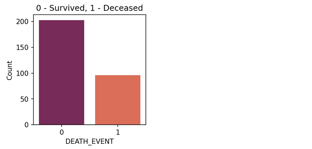
From the plot, the recovered rate is almost double the deceased rate of the patients. Here, the data is a bit unbalanced. Generally, The SMOTE technique is used to make the data balanced. As of now, Let’s keep it like that.

2. Check the categorical variables, and how they are behaving corresponding to the target variable.

Code:

plt.figure(figsize=(4,3),dpi=150)
sns.countplot(x=”sex”,hue=’DEATH_EVENT’, data=df,palette=’viridis’)
plt.ylabel(“Count”)
plt.xlabel(“Gender”)
plt.title(‘0 — Female, 1 — Male’)
plt.show()

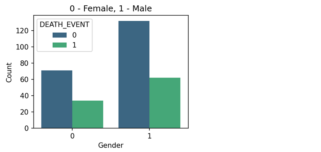
From the plot, The number of male patients is almost double of female patients. We can conclude that the death rate is almost half the survival rate in both categories.

Code:

plt.figure(figsize=(4,3),dpi=150)
sns.countplot(x=”high_blood_pressure”,hue=’DEATH_EVENT’, data=df)
plt.ylabel(“Count”)
plt.xlabel(“Blood Pressure”)
plt.show()

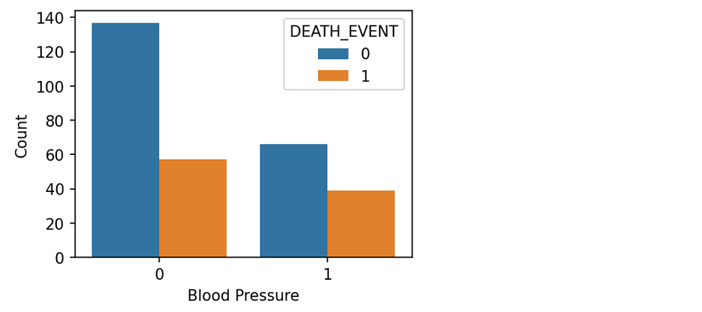
From the plot, The number of patients not having hypertension is almost double of the patients having hypertension. We can conclude that there is a more chance of heart failure when a person is having high blood pressure.

Code:

plt.figure(figsize=(4,3),dpi=150)
sns.countplot(x=”smoking”,hue=’DEATH_EVENT’, data=df,palette=’mako’)
plt.ylabel(“Count”)
plt.show()

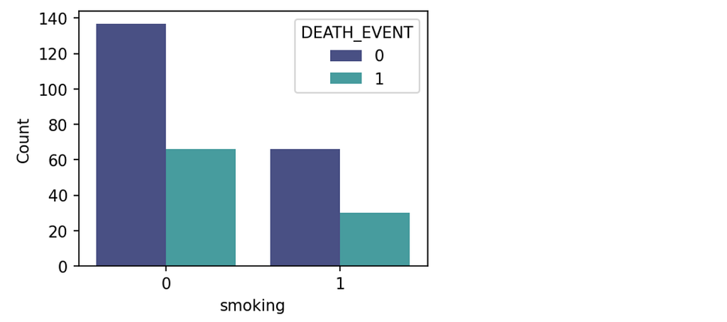
From the plot, The number of patients not smoking is almost double of the smoking patients. We can conclude that the death rate is almost half the survival rate in both categories.

3. Check the continuous variables, and how their trends and patterns are distributed.

Code:

print(‘The mean value is’, df[‘age’].mean())
print(‘The kurtosis value is’, df[‘age’].kurt())
plt.figure(figsize=(4,3),dpi=150)
sns.distplot(df[‘age’],color=’orange’)
plt.show()

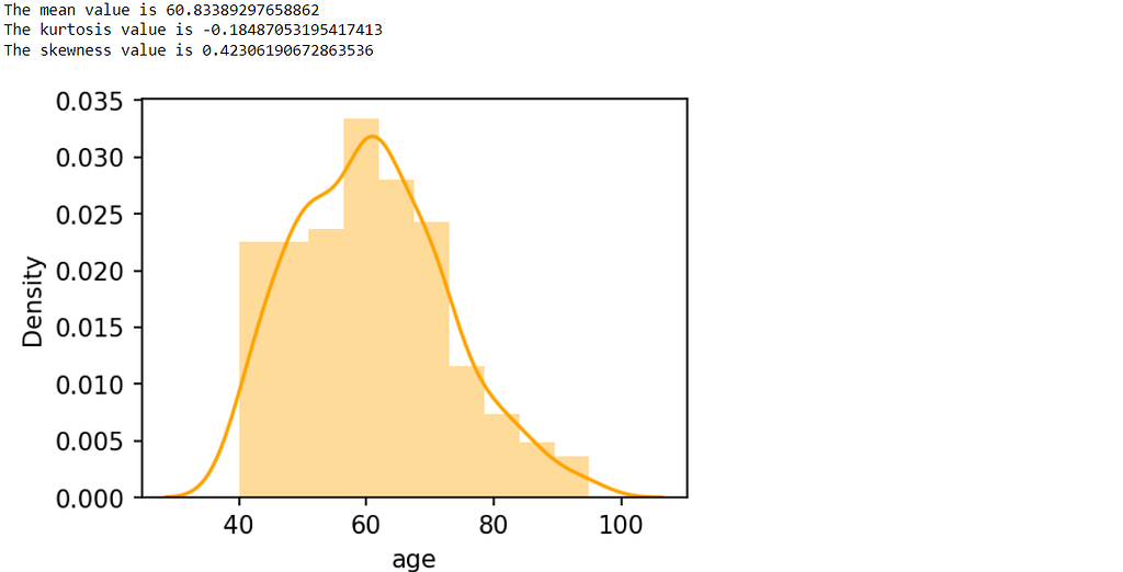
From the graph, we can say the average value of a patient’s age is around 60 years old and the range is in between 40 to 95 years. The skewness value is positive, which means there are more number of observation present on the right side of the graph and conclude that more people are younger than 60 years.

print('The mean value is', df['serum_sodium'].mean())
print('The kurtosis value is', df['serum_sodium'].kurt())
print('The skewness value is', df['serum_sodium'].skew())
plt.figure(figsize=(4,3),dpi=150)
sns.distplot(df['serum_sodium'],color='black')
plt.show()

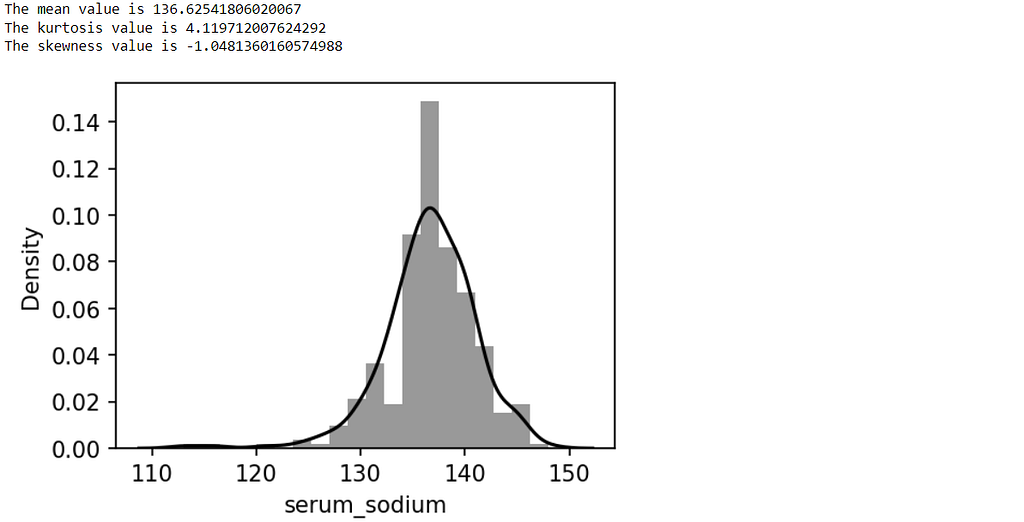
From the above plot, we can say the average value of the serum sodium level in most of the patients is 136 (mEq/L) and most of the patients are having a value greater than that.

Code:

plt.figure(figsize=(4,3),dpi=150)
sns.boxplot(data=df,x='DEATH_EVENT',y='platelets')
plt.show()

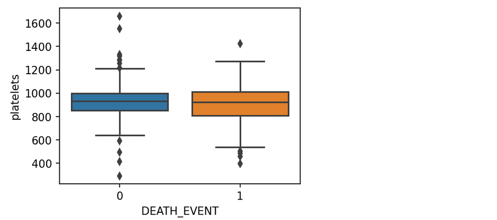
From the above graph, we can say there are more extreme values present in the count of survived patients. The average values of both categories are almost the same. Looks like, There are some outliers present in this feature as well these need to be handled.

4. Let’s go through the multi-variate analysis to check how the features are exhibiting the trends for one another. It can be possible with the help of heatmap and the pairplot methods. The heatmap method determines how strong the variables are related to each other. Whereas the pairplot method determines what does shape of relation between variables looks like.

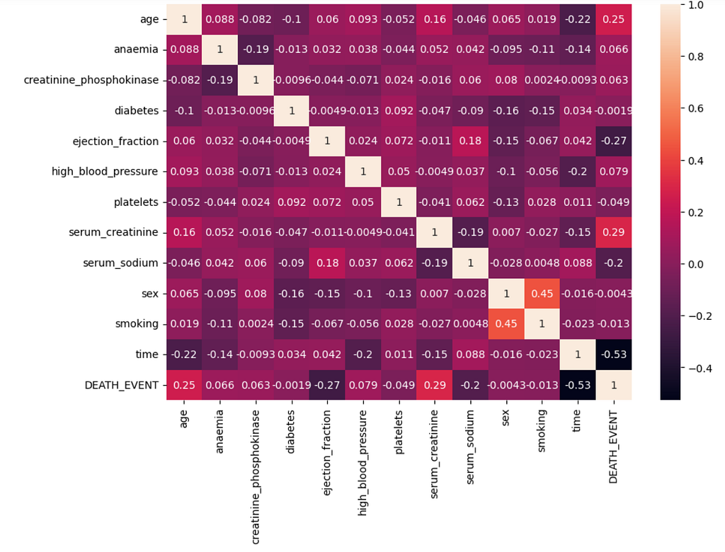
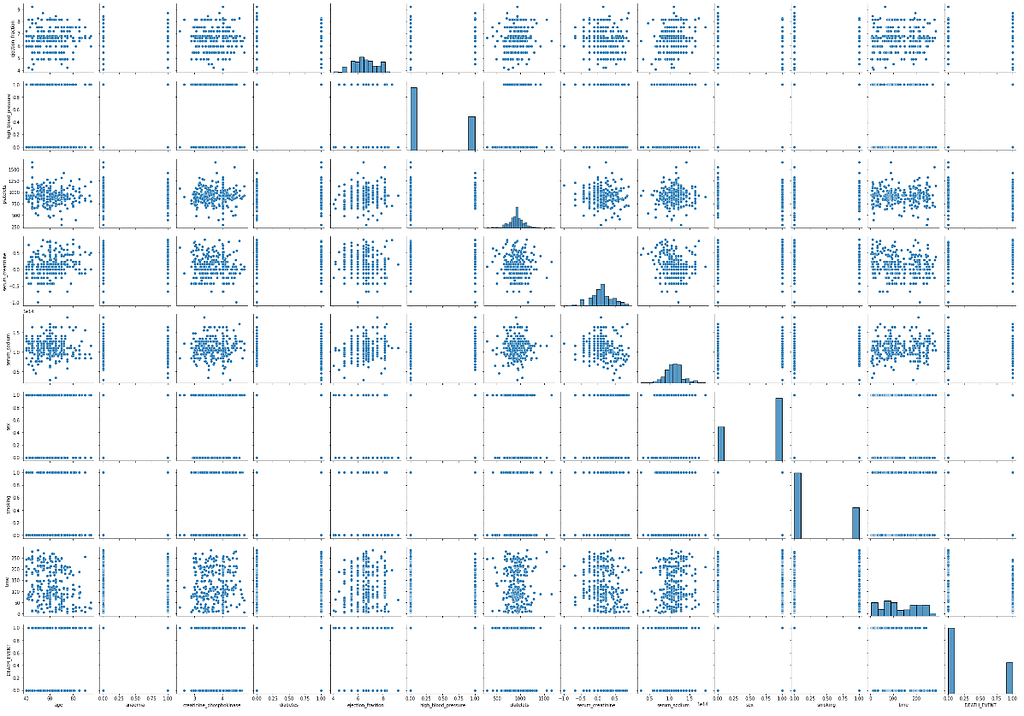
From the plots, we can say the features are not strongly correlated to each other. So here, there need to worry about the co-variance problem and can consider all the features to predict the output.

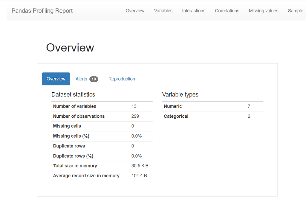
5. Finally, In Exploratory Data Analysis there is a magical and powerful package that would automatically do all of the things we have gone through so far which is the pandas_profiling package. It is better to prefer automated EDA when you have less time and want to concentrate much on the model. I’m attaching the first page of the HTML template generated by the ProfileReport method and you could explore it later on.

Code:

from pandas_profiling import ProfileReport
profile = ProfileReport(df)
profile

Data Pre-Processing

Outlier Detection

Outliers in the dataset can drastically impact the model output from the expected result. So, It’s better to detect them first with the help of any techniques like the Interquartile range method, DBSCAN, etc. The IQR method considers the values that are less than the lower tail and the values that are greater than the upper tail as outliers.

Code:

def iqr_method(data_frame,column_name):
    q1 = data_frame[column_name].quantile(0.25)
    q3 = data_frame[column_name].quantile(0.75)
    iqr = q3-q1
    Lower_tail = q1 - 1.5 * iqr
    Upper_tail = q3 + 1.5 * iqr
    return(pd.concat([data_frame[data_frame[column_name]<Lower_tail],data_frame[data_frame[column_name]>Upper_tail]]))
iqr_method(df[:],'serum_sodium')

The above are the outliers present in the serum_sodium. Similarly, there are some outliers present in the other features as well.

Outlier Handling

So, we can transform the variable that eliminates the outliers. Because it’s better not to delete the entries as the dataset is of less size. Here, I used the boxcox transformation to handle the outliers and wrote a code for automatic handling of the outliers.

Code:

def automated_handling_outliers(df1):
    outlier_feature_names=[]
    for i in df1.columns:
        if len(iqr_method(df1[:],i))>0:
            print(i)
            outlier_feature_names.append(i)
    for i in outlier_feature_names:
        df1[i],fitted_lambda= scipy.stats.boxcox(df1[i] ,lmbda=None)
    return(df1)
df=automated_handling_outliers(df[:])

Split the Dataset

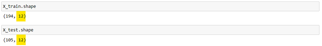
The purpose of this step is to split the dataset into test and train datasets so that there would be different data present for model training and prediction. This can be done by using the train_test_split function. Generally, the (70–30)% or (60–40)% ratio is considered to split the dataset into train and test data.

Code:

X = df.drop('DEATH_EVENT',axis=1)
y = df['DEATH_EVENT']
from sklearn.model_selection import train_test_split
X_train, X_test, y_train, y_test = train_test_split(X,y,test_size=0.35,random_state=101)

Scale the Data

Data scaling is an essential step in data pre-processing steps. If the data have various magnitude ranges, then it would be difficult for the ANN model to set the weights and modify them to get the best result. So here, the min-max scaler is used to bring the entire data into a certain range between 0 to 1 at the same time it preserves the behavior (trend) of the data.

Code:

from sklearn.preprocessing import MinMaxScaler
scaler = MinMaxScaler()
X_train= scaler.fit_transform(X_train)
X_test = scaler.transform(X_test)

Create an ANN Model

To create a model, we have some powerful libraries like the Tensorflow and Keras packages that make this process very simple within less time. The Keras package would make things easy to work upon because it has all the functionalities you just need to define them and use them wherever you want. Previously, these packages are separate but now they are integrated into the recent version of the TensorFlow package. Let’s import these packages to create a model.

Code:

from tensorflow.keras.models import Sequential
from tensorflow.keras.layers import Dense
from tensorflow.keras.optimizers import Adam
from tensorflow.keras.callbacks import EarlyStopping

Once the packages and functionalities are imported, create a model using the functionalities. First, we have to create a model layout that would work sequentially.

Code:

model = Sequential()

Now, add the dense layers to the sequential model. Each dense layer has neurons and each neuron has a corresponding activation function. Always an input layer would come first with the neurons equal to the number of features in the dataset. Generally, most people consider the Rectified linear unit (relu) as the activation function for all the neurons on that layer unless it is an output layer.

Add the hidden layers as your wish, there would be some rules for that as well. Most people suggest having the number of neurons in 2 power like (16,32,64,..) with the relu activation functions in a single layer. For the output layer, we can have one neuron with the sigmoid activation function as this is binary classification.

Code:

model = Sequential()
model.add(Dense(12,activation='relu'))
model.add(Dense(24,activation='relu'))
model.add(Dense(24,activation='relu'))
model.add(Dense(1,activation='sigmoid'))

Then, compile the model by defining the loss function and optimizer. Here, the loss function is considered binary_crossentropy as this is a binary classification problem and optimizer as adam for the optimum performance of the model.

Code:

model.compile(loss='binary_crossentropy', optimizer='adam')

Train and Evaluate the Model

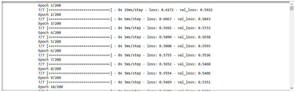
Training the model is done with the help of the fit method by giving the training dataset of features and the target variable. Here to this method, we can pass the validation data as a parameter then that would determine the validation loss while model training. In this case, test data can be taken for validation purposes.

There is one more important parameter epoch. If one epoch is completed that means the model goes through the trained data for one time. That value can be set for a large value but not too large. If the epoch parameter is set to a large value then the overfitting problem might occur.

Code:

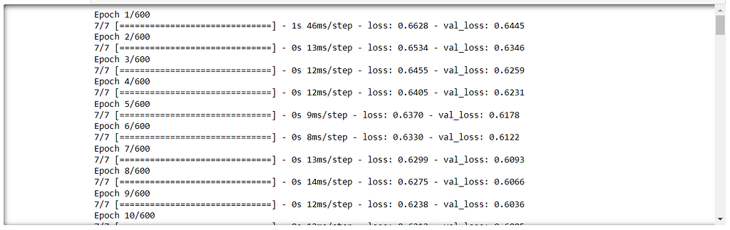
model.fit(x=X_train,y=y_train.values,validation_data=(X_test,y_test.values),epochs=200)

Once the model gets trained on the training dataset, it’s better to check the history of the model which means its performance on the validation data.

Code:

model_loss_1 = pd.DataFrame(model.history.history)
plt.figure(figsize=(4,3),dpi=150)
plt.plot(model_loss_1['loss'],color='r',data=model_loss_1,label='loss')
plt.plot(model_loss_1['val_loss'],color='g',data=model_loss_1,label='val_loss')
plt.legend()
plt.show()

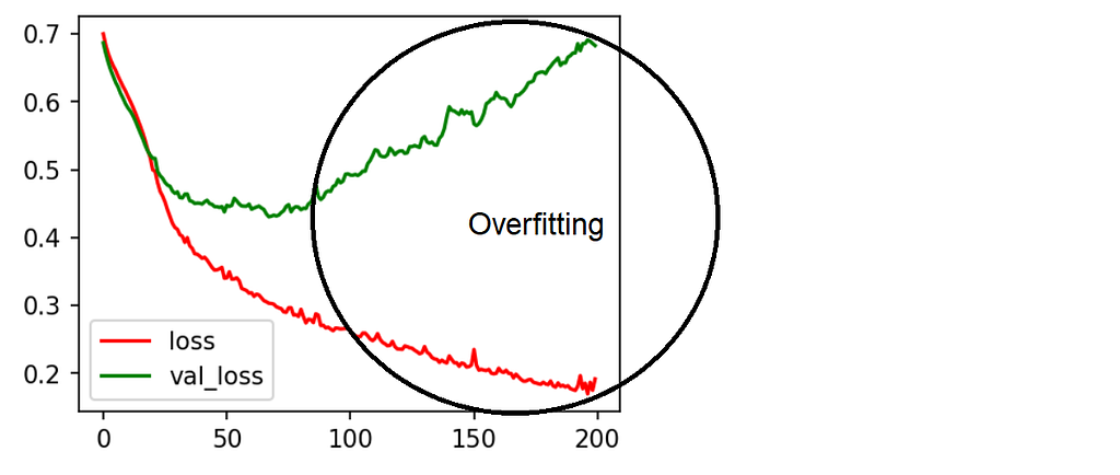
From the graph, we can say that the training loss and validation loss both decreased for a while. After the threshold value of epochs, the validation loss started increasing whereas the training loss remain decreasing. This problem is called Overfitting.

To overcome the above problem, there is a concept called Early Stopping from the callbacks in Keras library. This early stopping technique stops the model from being trained furthermore based on the given parameter. Let’s implement this by recreating the model. Define the early stopping method by setting the monitor parameter to validation loss. Here, the patience parameter is nothing but how long the model has to wait and continue the training even after noticing the drastic changes in the monitoring parameter.

Code:

model = Sequential()
model.add(Dense(units=12,activation='relu'))
model.add(Dense(units=24,activation='relu'))
model.add(Dense(units=24,activation='relu'))
model.add(Dense(units=1,activation='sigmoid'))
model.compile(loss='binary_crossentropy', optimizer='adam')
early_stop = EarlyStopping(monitor='val_loss', mode='min', verbose=1, patience=2)
model.fit(x=X_train, y=y_train,epochs=600,validation_data=(X_test, y_test),verbose=1,callbacks=[early_stop])

When you add the functionality of early stopping to the model, it does not depend on the number of the epochs even if it is a large number. Now, Let’s check the history of the model by plotting the training loss and validation loss of the model.

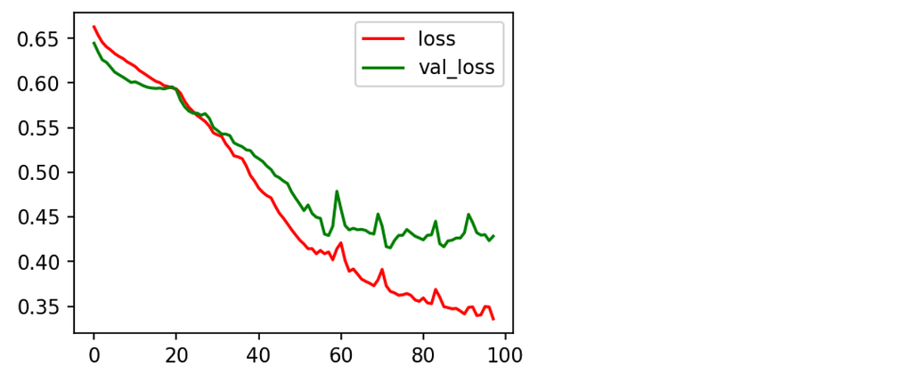
From the graph, we can interpret that the model training has stopped for around 100 epochs. There is no overfitting that has occurred during the model training.

Predict the Data

This step can be done with the help of the fit method where you would test data as the parameter to the model.

Code:

df_y=pd.DataFrame()
df_y['y']=y_test
df_y['y_hat']=model.predict(X_test)
df_y['y_hat']=df_y['y_hat'].apply(lambda x: 1 if x>0.5 else 0)

Let’s import the modules that determine the score of accuracy, precision, and recall of the model from the sklearn package.

Code:

print("Accuracy Score of the model:",accuracy_score(df_y['y'],df_y['y_hat']))
print("Precision Score of the model:",precision_score(df_y['y'],df_y['y_hat']))
print("Recall Score of the model:",recall_score(df_y['y'],df_y['y_hat']))
print(classification_report(df_y['y'],df_y['y_hat']))

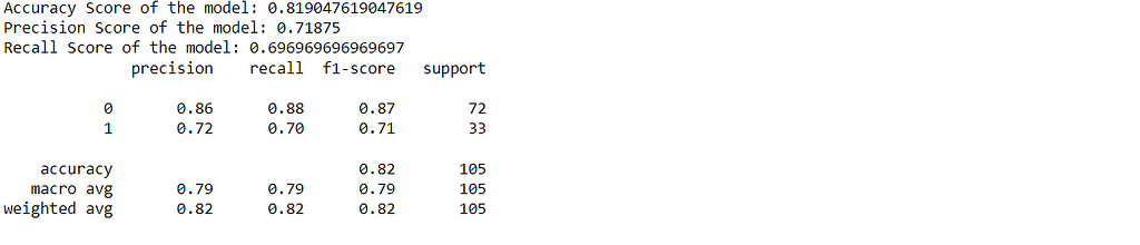
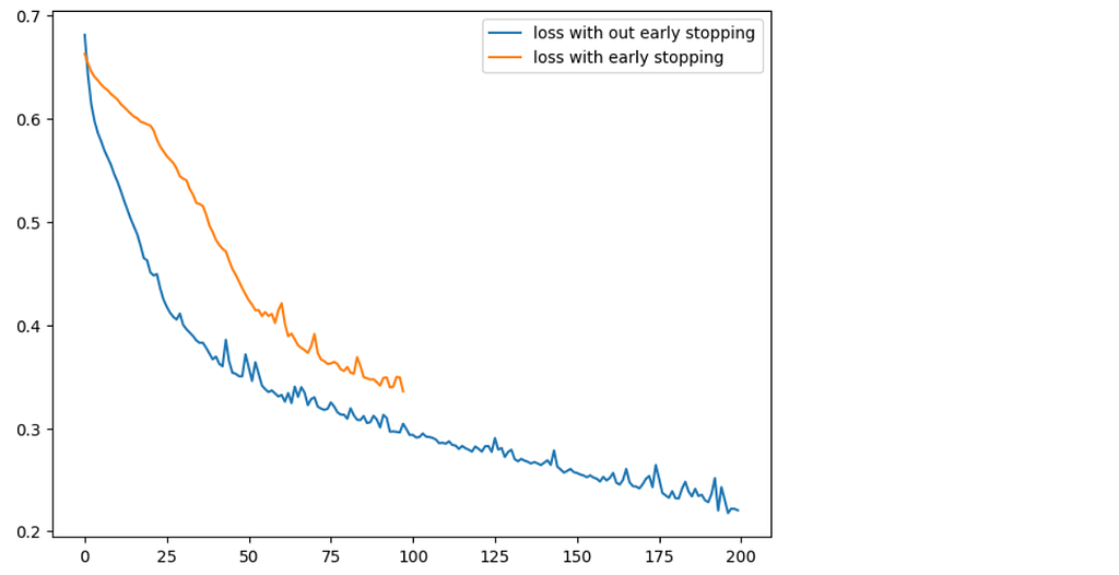
Well, I have got an overall accuracy of 82% that’s not bad. You might get different accuracy based on the data preprocessing and tunning of the model. In addition to that, You can try integrating dropout layers as well in between the model to reduce the chance of the model getting overfitted. Before concluding, let’s compare the performance of the model with early stopping and without early stopping by plotting its history of it.

Code:

plt.figure(figsize=(8,6),dpi=100)
plt.plot(model_loss_1['loss'],data=model_loss_1,label='loss with out early stopping')
plt.plot(model_loss_2['loss'],data=model_loss_2,label='loss with early stopping')
plt.legend()
plt.show()

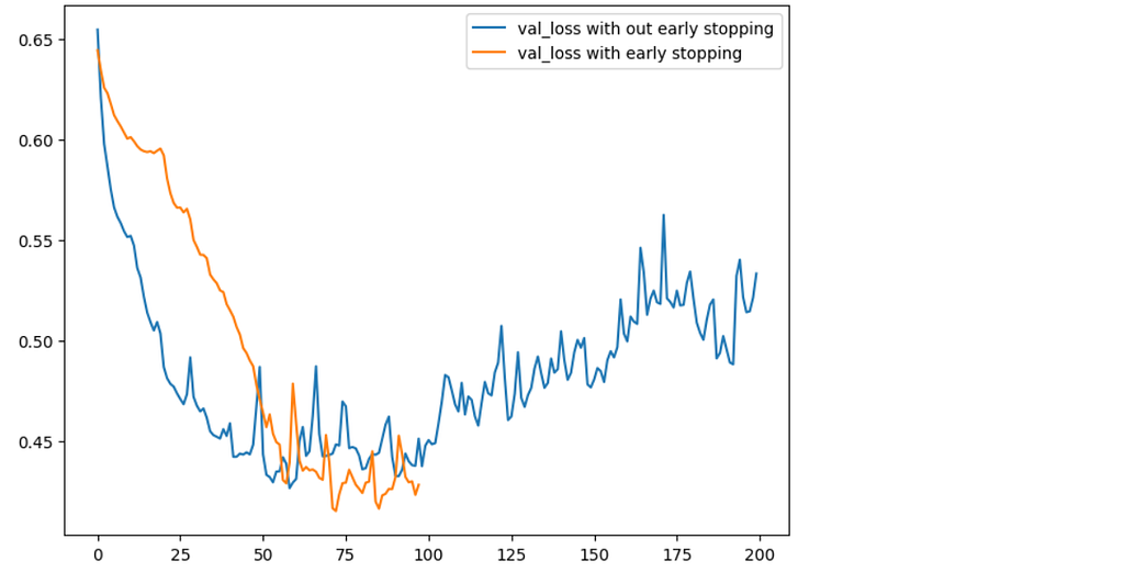
Code:

plt.figure(figsize=(8,6),dpi=100)
plt.plot(model_loss_1['val_loss'],data=model_loss_1,label='val_loss with out early stopping')
plt.plot(model_loss_2['val_loss'],data=model_loss_2,label='val_loss with early stopping')
plt.legend()
plt.show()

Source Code

Heart-Failure-Prediction-Using-ANN/DL_medium.ipynb at main · balupeddireddy08/Heart-Failure-Prediction-Using-ANN

Conclusion

So, I would like to say that they're many cool applications out there to work on and you can implement them with ANN. I thought of including some more interesting things in the article but it’s already lengthy. I will try to add those things in the coming article.

I hope you have an interesting read and this article is useful for you…🤝

Let me know if you have any doubts and correct me if anything is wrong with the article. All suggestions are accepted…✌

Happy Learning😎

---

A Short Journey To Deep Learning was originally published in Towards AI on Medium, where people are continuing the conversation by highlighting and responding to this story.

Join thousands of data leaders on the AI newsletter. It’s free, we don’t spam, and we never share your email address. Keep up to date with the latest work in AI. From research to projects and ideas. If you are building an AI startup, an AI-related product, or a service, we invite you to consider becoming a sponsor.

Published via Towards AI