


2D Path Planning With CNN
Last Updated on January 22, 2023 by Editorial Team
Author(s): Davide Caffagni
Originally published on Towards AI.
A convolutional neural network (CNN) is a popular model for solving tasks like image classification, segmentation, object detection, etc. This is an experiment to assess its application to solve simple 2D path planning problems. The programming language used is Python, with PyTorch, NumPy, and OpenCV as the main libraries. You can find the source code on my GitHub.
The task
Simply put, given an occupancy grid map, 2D path planning is about finding the shortest possible path to follow from a given starting point to a desired target position (goal), avoiding any obstacle during the trajectory. Robotics is one of the main fields in which path planning is critical. Algorithms like A*, D*, D* lite, and related variants were developed to solve this kind of problem. Nowadays, artificial intelligence (AI), especially with reinforcement learning, is widely used to account for that. Indeed CNNs are usually the backbone of some reinforcement learning algorithms. This experiment tries to address simple path-planning instances using a convolutional neural network solely.
The dataset
The main problem I faced was (as always in machine learning) where to find the data. I’ve ended up creating my own dataset for path planning by making random 2d maps. The process of creating a map is very simple:
- Let’s start with a square empty matrix M of 100×100 pixels.
- For each item (pixel) in the matrix, draw a random number r from 0 to 1 from a uniform distribution. If r > diff, then set that pixel to 1; otherwise, set it to 0. Here diff is a parameter representing the probability for a pixel of being an obstacle (i.e., a position that can’t be traversed) and thus, it’s proportional to the difficulty of finding a feasible path over that map.
- Then let’s exploit the opening morphological operator to get a “blocky” effect that better resembles real occupancy grid maps. By varying the size of the morphological structuring element and the diff parameter, we are able to generate maps with different levels of difficulty.
- Next, for each map, we have to choose 2 different positions: the start (s) and the goal (g). That choice is again casual, but this time we have to ensure that the euclidean distance between s and g is greater than a given threshold to make the instance challenging. Otherwise, our network won’t learn much from it.
- Finally, we need to find the shortest path from s to g. That will be the ground truth for our training. To this purpose, I’ve used the popular D* lite algorithm. In particular, I’ve written a custom implementation that constrains the solution to keep a margin of at least 1 free cell from any obstacle. The reason for that is simply that I was working on a robotic project where we required such a modification since our robot was often bumping against walls while following the original D* lite trajectory. By using the margin constraint, we were able to overcome the issue. And given that this CNN was (initially) thought to be used on that very same robot, I decided to keep our custom implementation.
The dataset comprises about 230k samples (170k for training, 50k for testing, and 15k for validation). Generating such an amount of data using the above process was found to be unfeasible with my commodity-level laptop. That’s why I’ve rewritten the customized D* lite implementation as a python extension module using the Boost c++ library. I have no benchmarks, but with the extension module, I was able to generate more than 10k samples/hour, while with the pure python implementation, the rate was about 1k samples/hour (on my old but gold Intel core i7–6500U with 8GB of RAM). The custom D* lite implementation is available here.
Notice that sometimes the goal position can appear to be placed on an obstacle. In those cases, the ground truth trajectory ends with the last feasible (i.e., a cell that is not an obstacle, a 0 in the matrix map) position closest to the goal. That’s another little difference from the original D* lite.
I made some simple checks on the data, for example, by deleting maps whose cosine similarity was very high and whose start and goal coordinates were too close.
I’ve uploaded the dataset on kaggle, where you can also find a simple notebook showing how to access samples. On the GitHub repository, you can also find a convenience script that allows you to build your own dataset from scratch.
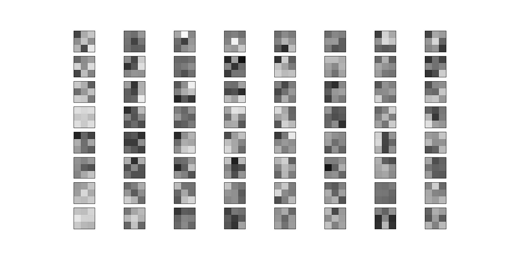
Model architecture
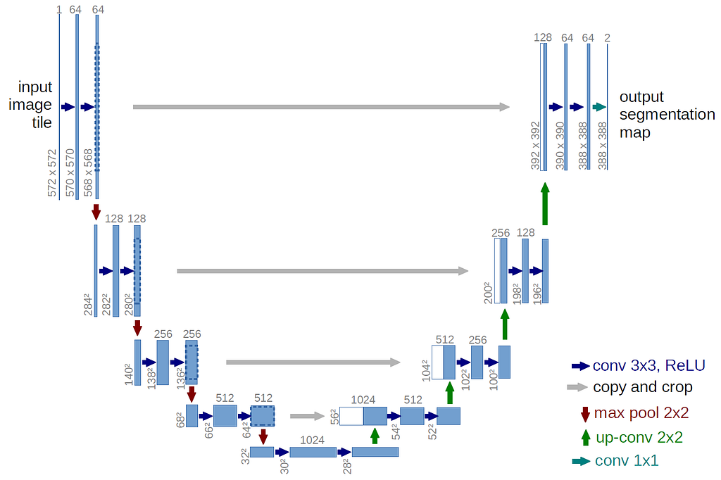
The model follows an encoder-decoder architecture, with a total of 20 convolutional layers divided into 3 blocks of convolution (the encoding part), followed by other 3 blocks of transpose convolution (the decoding part). Each block consists of 3 3×3 convolutional layers, with batch normalization and ReLU activation between each of them. Finally, there are other 2 conv layers, plus the output layer. From a high-level point of view, the encoder's objective is to find out a compressed yet relevant representation of the input. Then, that will be fed to the decoder part, which will try to reconstruct the same input map, but this time embedding useful information that should help find the optimal path from s to g.
The expected inputs of this network are:
- map: a [n, 3, 100, 100] tensor representing the occupancy grid maps. Hereafter, n is the batch size. Notice that the number of channels is 3 rather than simply 1. More on this later.
- start: a [n, 2] tensor containing the coordinates of the starting point s in each map
- goal: a [n, 2] tensor containing the coordinates of the target point g in each map
The output layer of the network applies the sigmoid function, effectively providing a “score map” in which each item has a value between 0 and 1 proportional to the probability of belonging to the shortest path from s to g. You can then reconstruct the path by starting from s and iteratively choosing the point with the highest score in the current 8-neighborhood. The process terminates once you find a point with the same coordinates as g. For the sake of efficiency, I’ve used bidirectional search algorithm for this purpose. This idea was inspired by this paper.

Between the encoder and decoder blocks of the model, I’ve inserted 2 skip connections. The model now really resembles the architecture (although being way smaller) of U-Net. Skip connections inject the output of a given hidden layer into other layers deeper in the network. They are employed when we care about details of the image being reconstructed (U-Net was indeed developed for medical image segmentation, where details are critical). In our task, the details we care about are the exact position of s, g, and all the obstacles that we must avoid in our trajectory. Initially, I didn’t include any skip connection, but I found later that this greatly improved the training convergence and the overall results of the model.
Training
I’ve trained the model for about 15 hours or 23 epochs on Google Colab. The loss function employed was the Mean Square Error (MSE) between the score map provided by the model and the ground truth (GT) map. The latter was obtained by creating a 100×100 matrix full of zeros and then adding a 1 in each location corresponding to a point belonging to the path obtained with the D* lite. Probably there are better choices than MSE, but I’ve stuck with it because of its simplicity and ease of use.
The learning rate was initially set to 0.001 with a CosineAnnealingWithWarmRestarts scheduler (slightly modified so as to decrease the max learning rate after each restart). The batch size was set to 160 samples.
As for regularization, I tried to apply gaussian blur to the input maps and also a small dropout at the first convolution layer. None of those techniques brought any relevant effect, so I dropped them in the end.
The problem with convolutions
At first, I fed the model using the occupancy grid map as they were. That is, the input was a tensor with shape [n, 1, 100, 100] (plus the start and goal positions). With this setup, I wasn’t able to achieve any satisfactory results. The loss stopped decreasing almost instantly. Consequently, the reconstructed paths were just random trajectories that completely missed the target position and went through the obstacles.
One of the key features of the convolution operator is that it is position invariance. What a convolutional filter learns is indeed a specific pattern of pixels that is recurrent in the data distribution it has been trained on. The patterns can, for instance, represent corners or vertical edges.
No matter what pattern a filter learns, the point is that it learns to recognize it independently from its position in the image. That’s for sure a desirable feature for tasks like image classification, where a pattern characterizing the target class could occur anywhere in the image. But in our case, the position is critical! We need the network to be very conscious about where the desired trajectory starts and where it ends.
Positional encoding to the rescue
Positional encoding is a technique for injecting information about the position of the data by embedding (usually by a simple sum) it in the data itself. It’s usually applied in natural language processing (NLP) to make a model conscious of the position of the words in a sentence. I thought something like that could be helpful for our task too.
The classical positional encoding (see the paper Attention Is All You Need) exploits a series of sinusoid to encode each position.
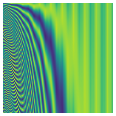
I ran some experiments by adding such a positional encoding to the input occupancy maps, but they didn’t go any better. Probably because by adding information about each possible position on the map, we are going against the position invariance property of a convolutional filter. The filters presented before are useless now since their weights should be adjusted to account for each and every possible different position on the input image. That’s, of course, unfeasible.
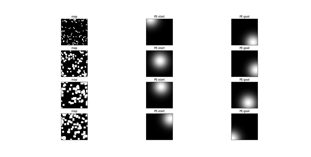
The idea I had is based on the observation that for path planning, we are not really interested in positions in absolute terms but only in relative scope. Specifically, we are interested in the position of each cell in the occupancy map with respect to the start point s and the goal point g. For instance, take a cell of coordinates (x, y). I don’t really care about knowing whether (x, y) is equal to (45, 89) rather than (0, 5). It should be way more useful to know that (x, y) is 34 cells away from s and 15 cells away from g.
What I’ve done is create 2 additional channels for each occupancy grid map that now has the shape [3, 100, 100] (not considering the batch size). The first channel is the vanilla map, as it was previously. The second channel represents a positional encoding that assigns to each pixel a value relative to the start position. Same story for the third one, but this time using the position. Such encodings are made by creating 2 feature maps from a 2d gaussian function centered on s and g, respectively. Sigma was chosen to be a fifth of the kernel size (as usual in gaussian filters). So in our case, sigma was 20, since the kernel size is equal to the side of the map, which is 100.

This time, while injecting useful information about the desired start and final locations of our trajectory, we partially restore the consistency with the positional invariance of our filters. Learnable patterns are now relying only on the distance with respect to a given point rather than on each possible location on the map. 2 equal patterns at the same distances from s or g will now cause the same activation of a filter. I found this little trick to be very effective in the convergence of the training.
Results and conclusions
I’ve tested the trained model over 51103 samples.
- 95% of the total test samples were able to provide a solution using the bidirectional search. That is, the algorithm managed to find a path from s to g in 48556 samples using the score map given by the model, while it wasn’t able to do so for the remaining 2547 ones.
- 87% of the total test samples presented a valid solution. That is, a trajectory from s to g that doesn’t traverse any obstacle (this value doesn’t account for the obstacle margin constraint of 1 cell).
- On the valid samples, the average error between the ground truth paths and the solutions offered by the model is 33 cells. That’s quite high, given that the maps are 100×100 cells. Errors range from a minimum of 0 (that is, “perfect” reconstruction of the ground truth path, found in 2491 samples) to a maximum of…745 cells (ok, this model won’t definitely replace the autopilot of a Tesla)
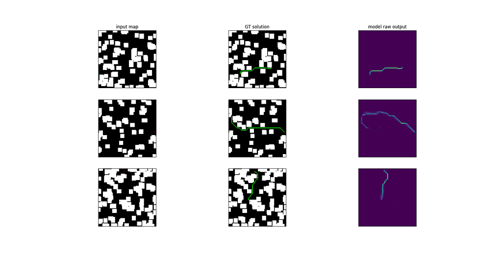
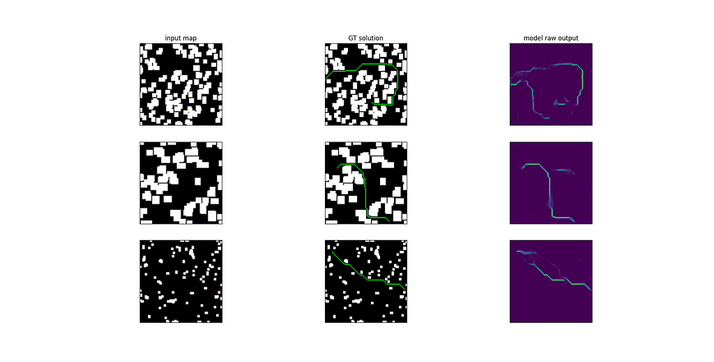
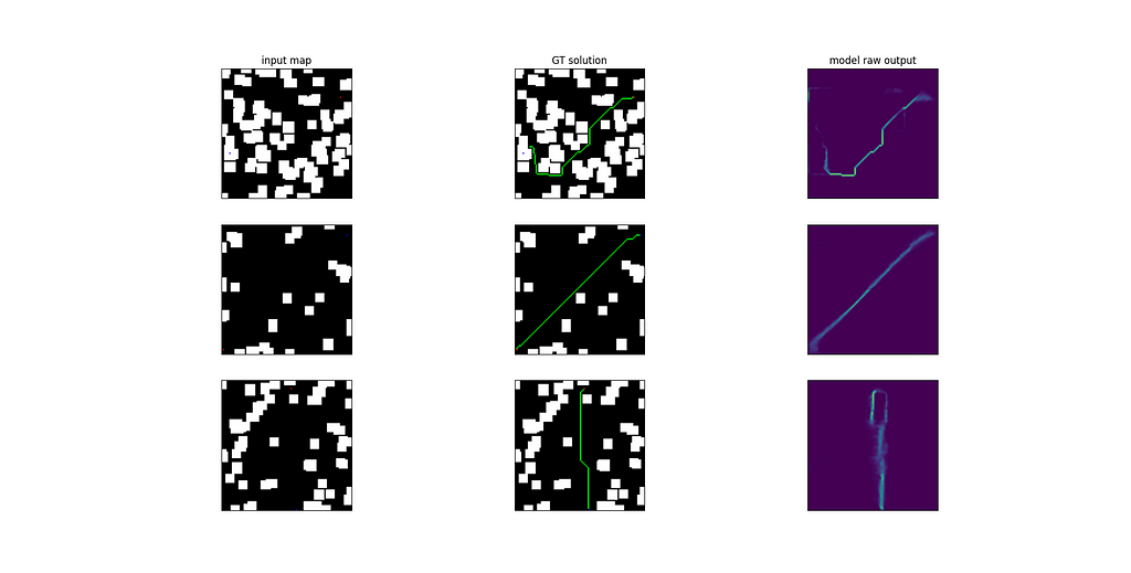
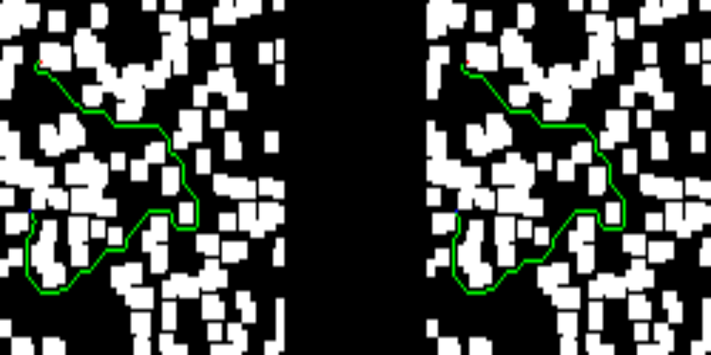
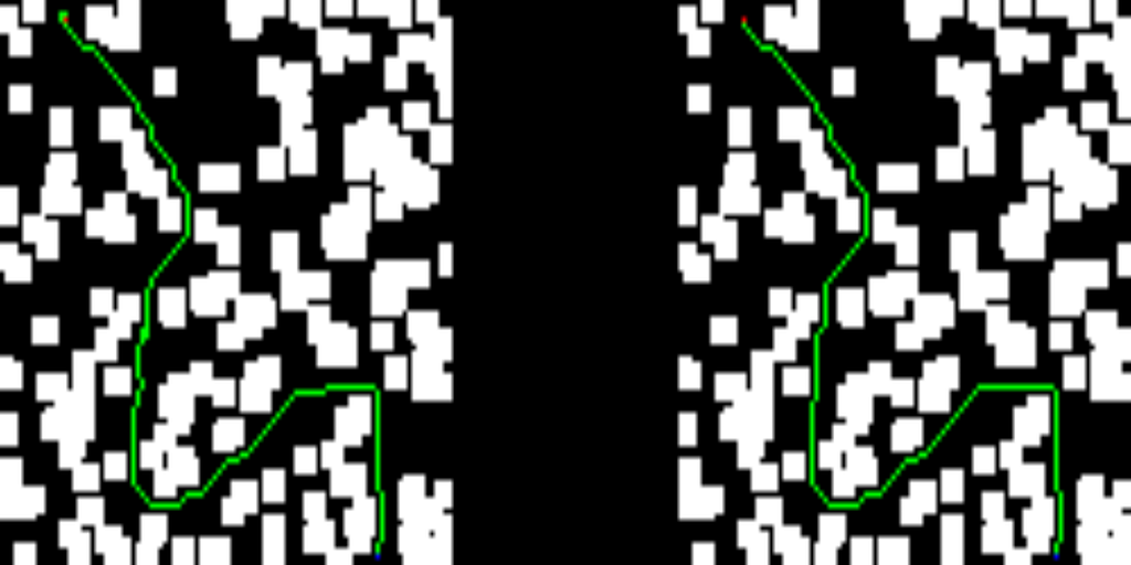
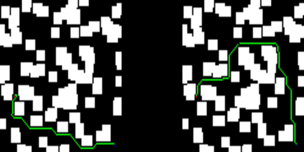
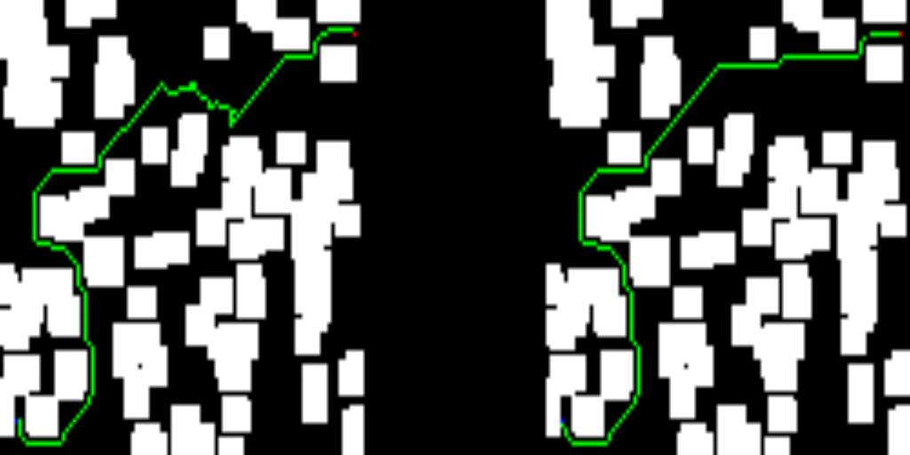
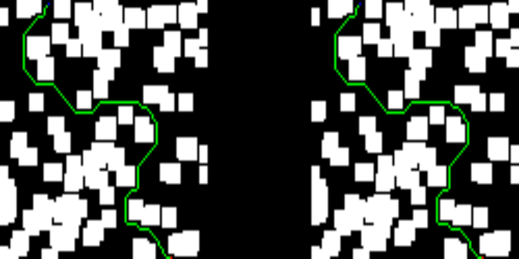
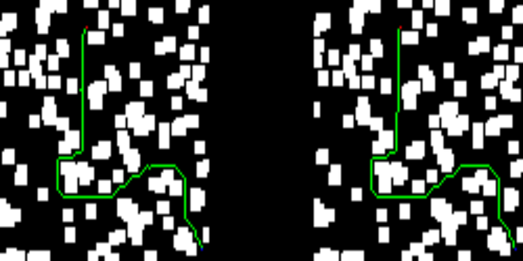
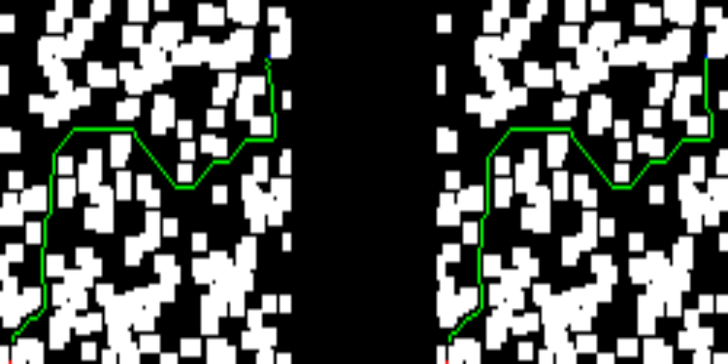
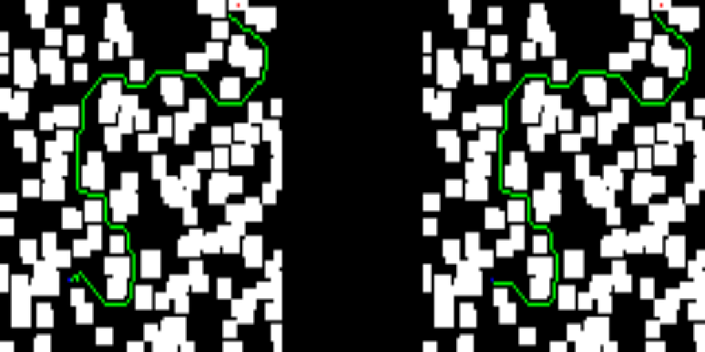
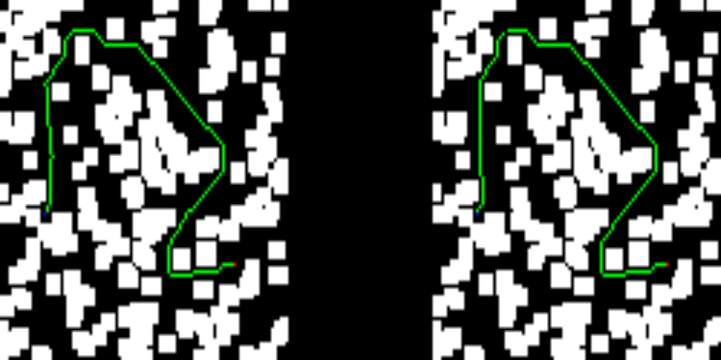
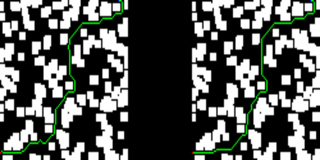
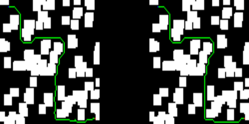
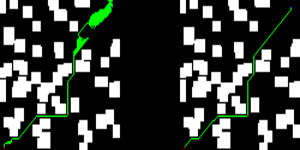
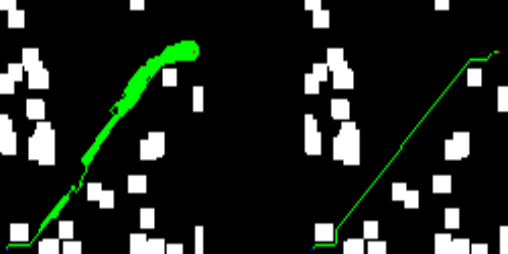
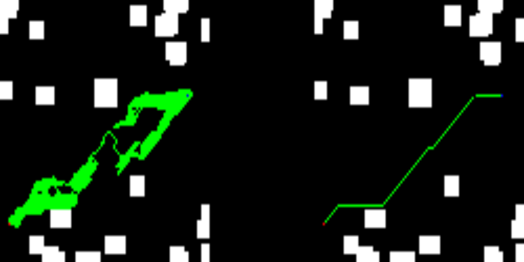
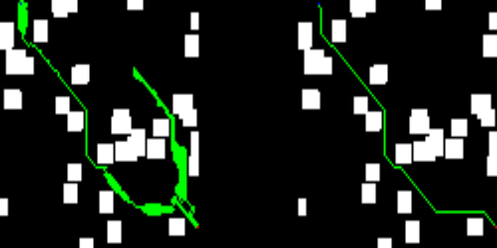
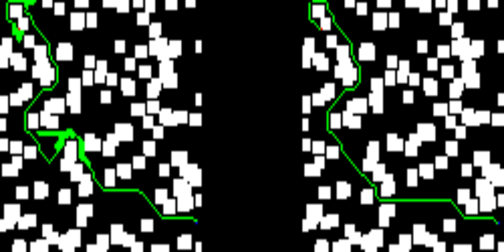
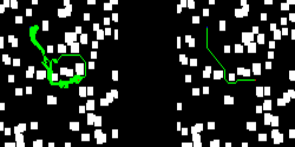
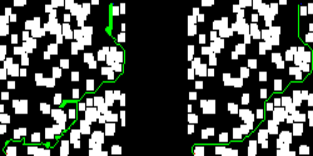
Right away, you’ll find some of the results from the test set. The left-hand side of the images depicts the solution provided by the trained network, while the right-hand side shows the solution of the D* lite algorithm.


If you’ve made it this far, let me thank you for your time. As you can see, this work is far from state-of-the-art results, but I had some fun while coding it, and I hope you enjoyed it as well.
2D Path Planning With CNN was originally published in Towards AI on Medium, where people are continuing the conversation by highlighting and responding to this story.
Join thousands of data leaders on the AI newsletter. Join over 80,000 subscribers and keep up to date with the latest developments in AI. From research to projects and ideas. If you are building an AI startup, an AI-related product, or a service, we invite you to consider becoming a sponsor.
Published via Towards AI
Towards AI Academy
We Build Enterprise-Grade AI. We'll Teach You to Master It Too.
15 engineers. 100,000+ students. Towards AI Academy teaches what actually survives production.
Start free — no commitment:
→ 6-Day Agentic AI Engineering Email Guide — one practical lesson per day
→ Agents Architecture Cheatsheet — 3 years of architecture decisions in 6 pages
Our courses:
→ AI Engineering Certification — 90+ lessons from project selection to deployed product. The most comprehensive practical LLM course out there.
→ Agent Engineering Course — Hands on with production agent architectures, memory, routing, and eval frameworks — built from real enterprise engagements.
→ AI for Work — Understand, evaluate, and apply AI for complex work tasks.
Note: Article content contains the views of the contributing authors and not Towards AI.
Related posts
Recent Posts
")


")


