Understanding the Universal Approximation Theorem

Last Updated on November 10, 2020 by Editorial Team

Author(s): Shiva Sankeerth Reddy

Let us take some time to understand the importance of Neural Networks

Neural networks are one of the most beautiful programming paradigms ever invented. In the conventional approach to programming, we tell the computer what to do, breaking big problems up into many small, precisely defined tasks that the computer can easily perform. By contrast, in a neural network, we don’t tell the computer how to solve our problem. Instead, it learns from observational data, figuring out its solution to the problem at hand.

Until recently we didn’t know how to train neural networks to surpass more traditional approaches, except for a few specialized problems. What changed was the discovery of techniques for learning in so-called deep neural networks. These techniques are now known as deep learning. They’ve been developed further, and today deep neural networks and deep learning achieve outstanding performance on many important problems in computer vision, speech recognition, and natural language processing.

That being said, let’s dive into the Universal Approximation Theorem.

Suppose someone has given you a wiggly function, say f(x) like below.

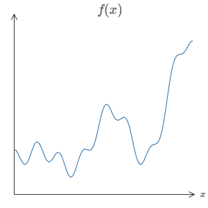
One of the striking features of using a Neural Network is that it can compute any function, no matter how complicated it is.

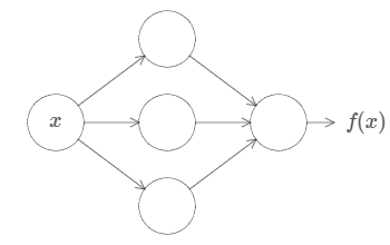
There is a guarantee that there will be a neural network for any function so that for every possible input, x, the value f(x)(or some close approximation) is output from the network, e.g.:

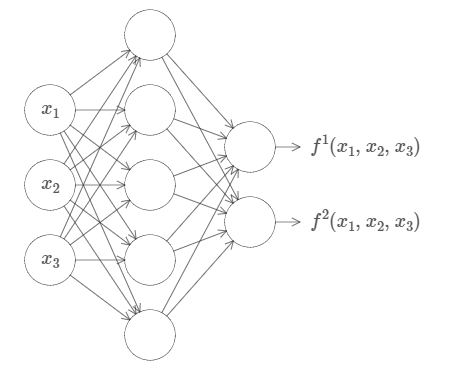
The above-said result holds even if the function has multiple inputs, f=f(x1,…, xm), and many outputs. For instance, here’s a network computing for a function with m=3 inputs and n=2 outputs:

This tells us that Neural networks have some kind of universality in them i.e. whatever the function may be that we want to compute, there is already a neural network available for it.

The universality theorem is well known by people who use neural networks. But why it’s true is not so widely understood.

Almost any process you can imagine can be thought of as function computation. Consider the problem of naming a piece of music based on a short sample of the piece. That can be thought of as computing a function. Or consider the problem of translating a Chinese text into English. Again, that can be thought of as computing a function.

Of course, just because we know a neural network exists that can (say) translate Chinese text into English, that doesn’t mean we have good techniques for constructing or even recognizing such a network. This limitation applies also to traditional universality theorems for models such as Boolean circuits.

Universality with one input and one output

let’s start by understanding how to construct a neural network which approximates a function with just one input and one output:

If observed keenly, this is the core of the problem of universality. Once we’ve understood this special case it’s pretty easy to extend to functions with many inputs and many outputs.

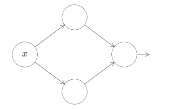
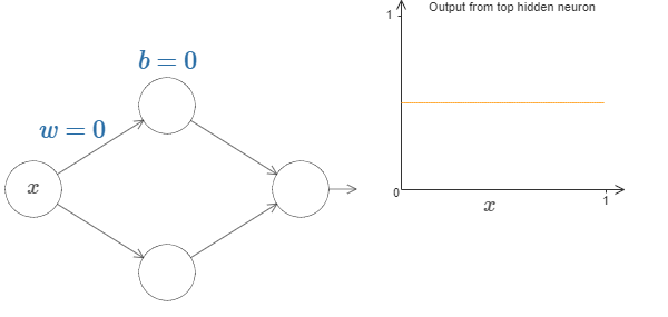
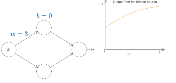
To build insight into how to construct a network to compute f, let’s start with a network containing just a single hidden layer, with two hidden neurons, and an output layer containing a single output neuron:

To get a feel for how components in the network work, let’s focus on the top hidden neuron. Let’s start with weight w = 0 and bias b = 0.

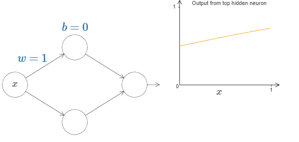
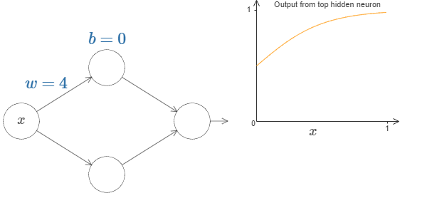
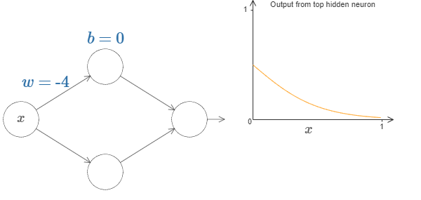
Let’s increase the weight ‘w’ by keeping bias constant. The below images show the function f(x) in 2D space for different values of weight ‘w’.

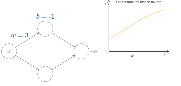
Now let’s change the bias by keeping weight constant.

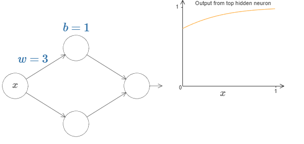
This visual representation of weights and bias in a simple neural network must have helped you to understand the intuition behind the Universal Approximation Theorem.

Many Input Variables

Let’s extend this approach to the case of many input variables. This may sound complicated, but all the ideas we need can be understood in the case of just two inputs. So let’s address the two-input case.

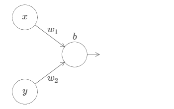
Here, we have inputs x and y, with corresponding weights w1 and w2, and a bias b on the neuron. Let’s set the weight w2 to 0, and then play around with the first weight, w1, and the bias, b, to see how they affect the output from the neuron:

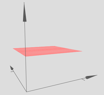
As you can see, with w2=0 the input y makes no difference to the output from the neuron. It’s as though x is the only input.

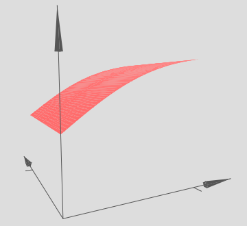
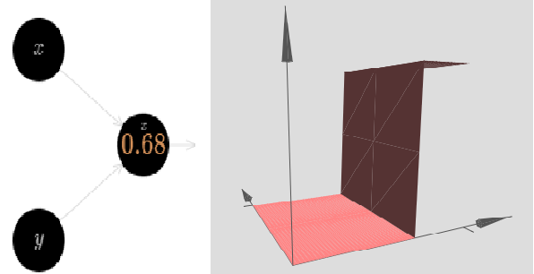
Let’s change the bias too to play with the graph and understand what’s happening.

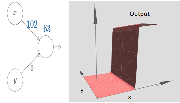
As the input weight gets larger the output approaches a step function. The difference is that now the step function is in three dimensions. Also as before, we can move the location of the step point around by modifying the bias. The actual location of the step point is Sx≡−b/w1

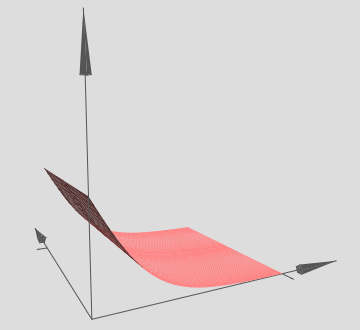
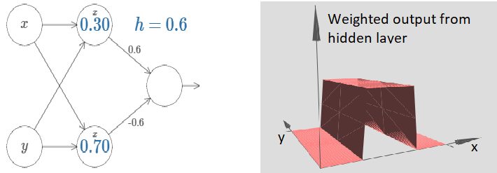
We can use the step functions we’ve just constructed to compute a three-dimensional bump function. To do this, we use two neurons, each computing a step function in the x-direction. Then we combine those step functions with weight h and −h, respectively, where h is the desired height of the bump. It’s all illustrated in the following diagram:

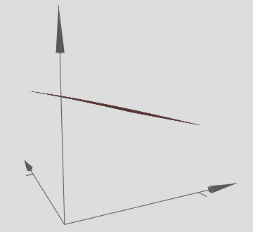
We’ve figured out how to make a bump function in the x-direction. Of course, we can easily make a bump function in the y-direction, by using two-step functions in the y-direction. Recall that we do this by making the weight large on the ‘y’ input, and the weight 0 on the x input. Here’s the result:

This looks nearly identical to the earlier network!

Let’s consider what happens when we add up two bump functions, one in the x-direction, the other in the y-direction, both of height h:

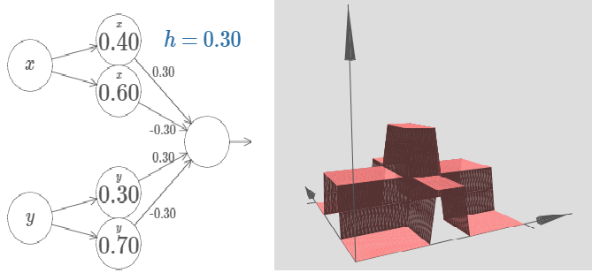
We can continue like this to approximate any kind of function. But we will end this discussion here and I will point you to some links in the bottom to let you play with these neural networks.

Conclusion

The explanation for universality we’ve discussed is certainly not a practical prescription for how to compute using neural networks!

Although the result isn’t directly useful in constructing networks, it’s important because it takes off the table the question of whether any particular function is computable using a neural network.

The answer to that question is always “yes”. So the right question to ask is not whether any particular function is computable, but rather what’s a good way to compute the function.

All the parts of this article are adapted from the book “Neural Networks and Deep Learning” by Michael Nielsen.

References:

1. A visual proof that neural nets can compute any function by Michael Nielson.
2. This article has been written as part of the assignment for Jovian.ml’s course “ZeroToGANs” offered in collaboration with freeCodeCamp.
3. Tensorflow’s Playground for intuitively understanding Neural networks.
4. Machine Learning Playground

---

Understanding the Universal Approximation Theorem was originally published in Towards AI — Multidisciplinary Science Journal on Medium, where people are continuing the conversation by highlighting and responding to this story.

Published via Towards AI