Understanding Artificial Neural Networks — Perceptron to Multi-layered Feedforward Neural Network

Last Updated on October 1, 2020 by Editorial Team

Author(s): Sanket Shinde

The transition of AI from classical machine learning to deep learning

This article will help you understand the transition of AI from classical machine learning to deep learning, starting from the basics of machine learning with its major – supervised and unsupervised learning to different regularization and optimization techniques.

The goal of this article is to introduce the major concepts of machine learning-what is machine learning? How does a machine learn by itself to do a particular task? How does it choose the essential features of the data that strongly contribute to the prediction of future events? How can we understand whether a machine has succeeded or failed in that?

In this article, we will discuss the foundations of artificial neural networks starting from perceptron to multi-layered feedforward neural networks. This article discusses the various stages of how to apply different transformation techniques for data preparation, how to train a neural network, and then validate and deploy a neural network for solving real-world problems.

In this article, we’re going to cover the following main topics:

· Understanding Machine Learning and Artificial Neural Network

· Feedforward Neural Network & Backpropagation Algorithm

· Evaluating and Tuning the Artificial Neural Network

· Classical Machine Learning vs Deep Learning

Understanding Machine Learning and Artificial Neural Network

This section starts with a brief overview of what is machine learning, its major types- supervised and unsupervised learning. Then we will understand the very evolution of artificial neural networks starting with how a biological neuron works. We’ll also discuss the design of artificial neurons with an understanding of deep neural networks with activation functions.

What is Machine Learning?

The term, Machine learning, has become a buzzword nowadays which refers to the ability of a machine to learn from the data without the help of the set of rules that are defined explicitly as like in the traditional rule-based algorithms. So definitely, if it learns from the data without any need for an explicit declaration of rules then it has to do with the experience from learning.

“Our way of learning always follows a curve of failures although it’s perfectly descendent, lastly it will converge to the extent of our hard work”

In the last decade of technology, machine learning techniques have become the common tools to automate the tasks that would have required huge efforts with the traditional rule-based algorithms.

In the traditional rule-based algorithms, the set of rules used to be defined to work on with a specific variety of data and could not be generalized to a large extent of data because of its specificity of working on only particular data. For example, if YouTube, a video sharing site decides to perform a copyright check on videos that are being uploaded on its server with a human operator, it will need a lot many people to execute this task of copyright check. But if YouTube chooses to do this with the help of some video processing algorithm then the task of copyright check would be easier but not robust as video processing algorithm possibly would work only on a set of videos that don’t have any kind of transformations like flip, rotate, crop, blur, etc. And it’s quite difficult to write a separate algorithm for individual transformation so the solution to this problem can be machine learning. In this case, a learning model is built by getting trained on data and identifying implicit features that uniquely signifies the data with which new data can be validated automatically.

Today, we are living in the era of machine-learning-based technologies; email services learn how to classify the emails into spam and ham; search engines learn what to recommend to the user based on their search history; banking systems are now able to sanction loans based on the creditworthiness of a customer. Prediction of heart disease based on clinical data, identifying voice commands, and forecasting annual rainfall are other significant tasks that machine learning facilitates.

One common problem with all of these applications is that a programmer cannot explicitly define the set of instructions for the task that needs to be performed due to the underlying complexity of the data; this was machine learning helps. It has made itself useful across industries like retail, banking, healthcare to the automobile industry for its ability to predict future events with significant accuracy.

In machine learning algorithms, the input is the experience in form of data and output is knowledge or wisdom gained with inductive inference which in turn helps to predict future events, so rather, machine learning is an art of experiential learning.

Let us start with a real-life experience of preparing a food dish with some cooking recipe, how do we prepare the food, let’s go through the process of making the delicious food, at first we collect all the ingredients that are needed for food preparation, as a naïve person in the cooking, we follow a cooking recipe which involves set of steps that need to be performed. Let us take an example of a famous dish of western India, poha, which needs many ingredients like beaten rice flakes, mustard, curry leaves, groundnuts, oil, salt, and others. Assume now, with all ingredients, we start making the poha as per the directions in the cooking recipe.

With this, we get a food dish, poha, but here comes the problem, when we taste it, we found that we have added more salt than required due to which poha became saltier. So, here is the first lesson that we got, every ingredient has a weight factor associated with it and if we are going to ignore that, we will not get the delicious taste as we expected. So, this has become the first learning experience of ours for making poha which has helped us in correcting the weight factors of individual ingredients, this time we will stay focused and will add the ingredients strictly as per their requirement, and due to which now, poha has become tastier than before.

This example of preparing food shows that we correct our decisions based on past learning experiences. So, it’s all about the learning experience that we get and according to which we take the corrective action. Because of this particular reason for human beings to adapt to the changing environment, the race of human beings has survived thousands of years until now. And this has become the sole reason for the evolution of the artificial neural network with which we can mimic the biological neural network of a human brain.

The artificial neural network works on the principle of the learning experience. The learning experience of a human being evolves based on improvements in his cognitive abilities through continuous corrective actions taken according to the changing environment.

Let us understand one of the popular machine learning algorithms, linear regression. Linear regression is a modeling approach to obtain a relationship between scalar dependent or target attribute and one or more independent attributes of the data. In order to study the linear regression, a linear equation forms the basis so let us start with a simple linear equation. A linear equation is an equation which when we plot on the graph, will give a straight line. The standard form of linear equation is,

y = mx + c

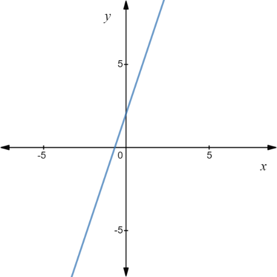
This relation shows that y is dependent on x that’s why y is called a dependent variable or target variable or response while x is called an independent variable or predictor or feature which helps in finding out y. While m represents the coefficient of x that tells the contribution of in finding y while c represents the bias factor. Let us try to understand this equation with an example, here we have taken m = 3, c = 2,

y = 3x + 2

We plot this equation on the graph for different values of y=1, 2, 3, 4, 5, 6 gives a straight line as shown in the following image,

In this simple linear equation, y=3x+2, there is only one independent variable, x. If a linear equation has more than one independent variable, it is called a multi-linear equation which is represented in the following form,

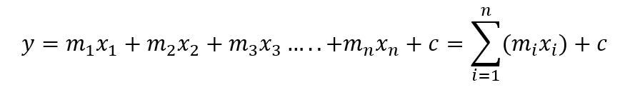
In the above equation, {m_1,m_2,m_3,…,m_n} represents set of coefficients of independent variables, {x_1,x_2,x_3,…,x_n} represents set of independent attributes contributing in finding out target variable, y.

Let us now formulate a multi-linear regression that uses multiples independent, explanatory attributes of data to predict the value for the target variable. The major goal of multi-linear regression is to build a prediction model by inferring a linear relationship between independent variables and a dependent, target variable. A multi-linear regression is represented as follows,

In the above equation, {β_1,β_2,β_3,…,β_n} represents set of coefficients of independent variables, {x_1,x_2,x_3,…,x_n} represents set of independent attributes contributing in finding out target variable, y.
A simple linear regression may help the analyst to build a prediction model based on a single independent variable while in multi-linear regression, it relies on multiple independent variables of data. Multi-linear regression has assumptions, a data is normally distributed with a mean of 0 and standard deviation σ, there exists a linear relationship between the independent variables and the dependent variable and there should not exist multicollinearity among the independent variable.

Let us take an example, a stock market analyst wants to build a prediction model for how different index movements affect the stock price of a company named ABC. In this formulation of the regression model, different indices will act as independent variables or predictors and a stock price of ABC acts as a response or target variable. So, in this scenario, a multilinear regression is worthy to determine a linear relationship between different independent variables and a target variable. A method of least squares is used to find the best fitting regression line for the set of data points by minimizing the sum of the squared errors which is a difference between an observed value and calculated value as shown in the following diagram,

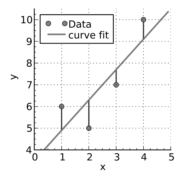
This is a method for curve fitting for regression analysis. Regression models can predict only continuous values while if we wish to predict discrete values or class or labels, classification algorithms are a good choice for the same.

Let us now take a brief overview of variants of machine learning algorithms- supervised and unsupervised machine learning.

Supervised Machine Learning

Supervised machine learning algorithm builds a learning model by getting trained on known data points and its known responses with which it could predict responses for unfamiliar data points. Regression and classification algorithms are major categories of supervised machine learning algorithms. The regression algorithm predicts continuous values by building the model based on relationships between the target variable and known data points. While the classification algorithm helps to predict discrete responses, it builds an inferred function based on the known labeled data, which in turn is used to predict the response for the unfamiliar data point. Naïve Bayes, decision trees, random forest, and support vector machines are important classification algorithms in machine learning.

Unsupervised Machine Learning

An unsupervised machine learning algorithm tries to infer patterns or a structure in a dataset that has unlabelled data points with minimal human supervision. It allows us to discover the inherent distribution of the dataset on its own. It mainly deals with unlabelled data. Cluster analysis and principal component analysis are major variants of unsupervised machine learning. In the neural networks, a self-organizing map (SOM)works on the basis of unsupervised learning with the capability of learning on its own without the need for any supervision.

What is an Artificial Neural Network?

The human brain has billions of neurons and trillions of synapses. The basic unit of the neural network is called a neuron, a neuron consists of dendrites having a tree-branch like structure as shown in the following diagram, that receives impulse signals from connected neurons, while axon transmits the signal from one neuron to another. Axon terminals are connected to dendrites of other neurons through synapses, the signal transmitted from the axon represents the electric pulse which is a response generated for the input signal.

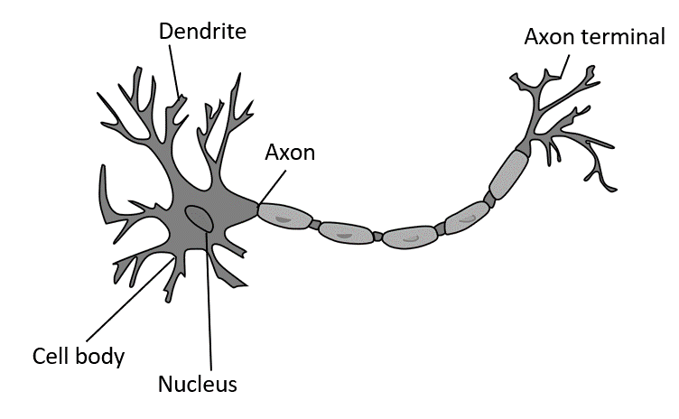
In short, a neuron checks for the total strength of different incoming signals to exceed the threshold and accordingly fires the electric pulse as a response. The neural network in the brain can learn more complex features than an artificial neural network due to the dense and fully connected multi-layered form of network.

The biological neural network helps human beings develop the ability to distinguish a cat from a dog. This ability to retain fine-grained details of the observed entity is gained by learning from the experiences.

An artificial neural network is the artificial form of a biological neural network. An artificial neural network is characterized by a weighted connection between layers of artificial neurons. These weighted connections can be fine-tuned by a learning algorithm that learns from the known data to improve the predictability of a neural network. A cost function is defined to make changes in the weights of connections between layers of neurons which is usually done with optimization techniques like gradient descent. We’ll discuss gradient descent more in the following sections. An artificial neuron as shown in the following figure represents the simplest form of artificial neural network.

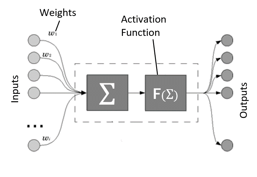
As shown in the above diagram it is clearly understood that information is feed forwarded from a set of input nodes to output nodes by aggregating the weighted features and passing to the activation function which in turns transforms the weighted sum of inputs of a neuron into a finite value based on some rule or requirements. The calculated score is matched with the observed value to fine-tune the network weights. This process continues until the difference between calculated and observed value minimizes drastically. Once this process of correcting network weights gets completed, we get the set of optimal network weights that are capable of learning complex relationships among sets of independent variables and a target or response variable.

Deep Neural Network

A deep neural network is a form of the artificial neural network which consists of a multi-layered network having more than one hidden layer between input and output layers. The deep neural network can construct a complex non-linear relationship model. Convolutional Neural Networks (CNNs) and Recurrent Neural Networks (RNNs) are typical examples of deep neural networks.

Deep neural networks are a form of a multi-layered feed-forward neural network. The major applications of deep neural networks are recommendation systems, visual recognition, clinical data analysis, financial fraud detection, language modeling, and many more. Deep Neural networks are characterized by their depth and the number of neuron layers in the network. More depth in layers of a neural network helps in higher convergence of a neural network for better predictability.

Activation Function

Let us now try to understand the activation function and its different variants in the next subsection. The activation functions play a major role in capturing the non-linear complex features of the data. The need for activation function arises to capture the collective representation of the features of the data.

An activation function is a transfer function of a neural network that allows the transformation of the weighted sum of inputs of a neuron into a finite range value. A simple activation function is called a linear activation function as it doesn’t perform any kind of transformation. Although its time-efficient, it doesn’t help to capture complex relationships between the features, so typical use of linear activation function is restricted to regression problems. Like linear activation functions, we have non-linear activation functions that are able to learn complex relationships between the features of the data which allows us to build more robust deep learning models.

An important requirement for an activation function is, it should not be computationally expensive as a modern neural network will possibly have thousands of activation nodes in it, which requires an activation function to be time-efficient. Basically, the main purpose of an artificial neural network is to learn the underlying complex features of the data.

The backpropagation is a gradient descent algorithm in which the network weights are adjusted in proportion to the negative gradient of the error function and backpropagated from the output layer to the input layer of a neural network. This process changing the weights continues until the overall error in the network reaches a minimum. As modern neural networks learn the complex relationships of data with the help of a backpropagation algorithm, it places a lot of computation strain on the activation nodes so it is highly recommended to use a time-efficient activation function for intermediate or hidden layers of neural network.

An activation function can be as simple as a weighted summation of input features or can be a transfer function which transforms the weighted summation of inputs into a finite range of values depending on the rule or threshold.

The following activation functions are mainly used for building neural network architectures. These are categorized into linear and non-linear activation functions.

Linear Activation Function

Let us consider the set of input features of the dataset are x1, x2, x3 represented as X. When these input features are fed to the neuron with weight multiplication gives the weighted sum of input features, Σ. The function, f(Σ) represents an activation function and ŷ represents the output score as shown in the following figure,

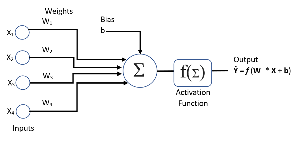
In the above diagram, we see that ŷ= f(Σ) but in the case of linear activation function, ŷ= f(Σ)=Σ

Linear activation functions don’t perform any transformation but are usable in solving regression problems where the output score ranges from -infinity to +infinity. The main challenge for the linear activation function is to learn the non-linear complex relationship between data elements features of a data set but as linear activation functions cannot capture the complex features of the dataset, the better solution is to use non-linear activation functions.

Non-linear Activation Function

Non-linear activation functions help to transform the weighted summation of input features into a finite range of values. Modern neural network architectures are increasingly using non-linear activation functions that help to learn complex data which in turn helps for accurate predictions. Non-linear functions allow better convergence of backpropagation (gradient descent) algorithm.

The following are the major non-linear activation functions used in neural architectures.

Sigmoid Function

The sigmoid activation function is defined as,

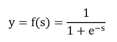
In this equation, s represents the weighted sum of input features; sigmoid function restricts the output value, y to a range of (0,1) as shown in the figure,

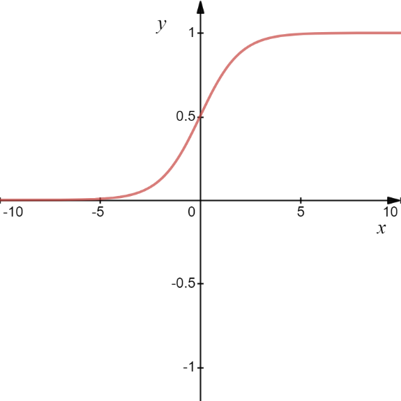
This activation function is computationally expensive so it’s typically used at the output layer but not in hidden layers of the neural network. For a very high or low value of, With the sigmoid function, when the value of s is too high or too low, the value of y does not change drastically. This results in the smaller change in the derivatives causing the problem of vanishing gradient which ultimately results in poor learning of neural networks as the neural network learns very slowly through gradual updation in the weights.

Hyperbolic Tangent Function (tanh)

This activation function bounds the output value to a finite range (-1,+1), it is the similarly-shaped non-linear activation function as shown in the following figure, as the sigmoid function

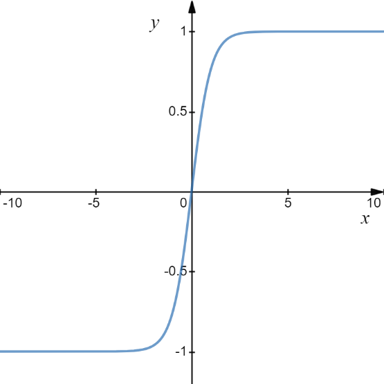
It has a better performance comparatively than the sigmoid function. Just like sigmoid, tanh function (hyperbolic tangent) has a problem of value saturation for higher or lower input values which converge to +1.0 and -1.0 respectively. Even if there is a significant change in input value it doesn’t change much as shown in the figure because of which, it becomes difficult for the backpropagation algorithm to make changes in the weights for better convergence.

In the learning phase of deep neural networks, the error is backpropagated through the neural layers for weight updation. But if the amount of error reduces drastically as it passes through more deep neural layers with the derivation of activation function then weights get updated very slowly, which results in slower learning of neural network. This is called the vanishing gradient (rate of change in weight updation). The vanishing gradient problem prevents the neural network from learning at a faster pace.

Rectified Linear Unit Function (RELU)

RELU is a highly recommended activation function for hidden layers in a neural network architecture as it is computationally efficient, it allows the neural network to converge quickly, and has a derivative function which helps in the backpropagation of errors through layers of neural network. It bounds the input value, s, to the range of a maximum of (0, s ) as shown in the following figure,

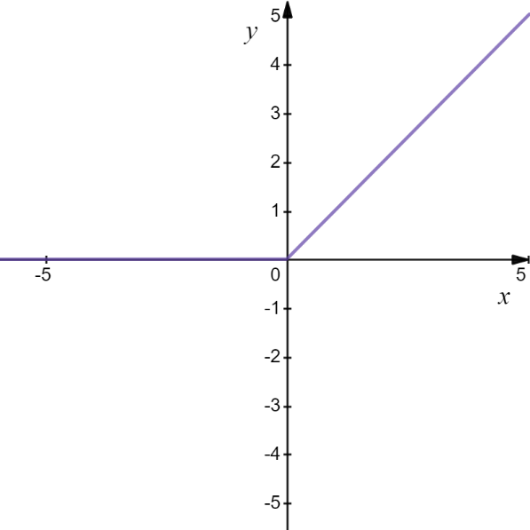
This activation function works linearly when the value of s is positive and it becomes non-linear when the value of s is negative and converges to zero. It’s highly recommended for architecting most of the variants of neural network architectures like multi-layered perceptron and convolutional neural networks.

Softmax Function

A Softmax is a highly popular non-linear activation function for solving multiclass classification problems, used only for the output layer to transform input into multiple class probability values in the range of (0,1).

While architecting a neural network, the selection of the activation function is a crucial decision. Experimenting with different activation functions with different neural layers can help us in better convergence of deep learning models.

In the next section, we will be learning more about the feedforward neural network with its major variant multi-layered perceptron along with the backpropagation algorithm for model optimization.

Feedforward Neural Network & Backpropagation Algorithm

Feedforward neural network forms a basis of advanced deep neural networks. In this section, we will take a brief overview of the feed-forward neural network with its major variant, multi-layered perceptron with a deep understanding of the backpropagation algorithm. The backpropagation algorithm updates the weights or parameters of the neural network based on the gradient of the loss function.

Feedforward Neural Network

A fully connected neural network represents a neural network having every node of each layer connected to every node of another layer starting from initial layers through hidden layers to the output layer. A fully connected neural network is also known as a dense neural network. Feedforward neural network is a form of artificial neural network where the flow of signals is feed forwarded without a formation of a cycle and the data from the input layer is fed to the output layer through a set of hidden layers.

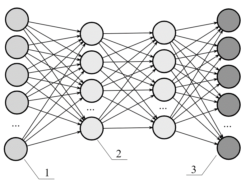
In this form of the neural network, the information flows from a set of input nodes (annotated as Set 1 in the above diagram) forwarded through hidden layers (as Set 2 in the diagram) to the output layer of neurons (annotated as Set 3 in the above a diagram), therefore, it is also referred as a Directed Acyclic Graph (DAG).

Multi-Layered Perceptron (MLP)

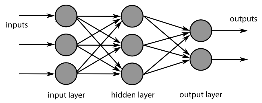
A multi-layer perceptron (MLP) is a form of feedforward neural network that consists of multiple layers of computation nodes that are connected in a feed-forward way. Each node in the neural layers has a connection to every neural node of the next layer; connections here represent weight assigned to the individual neural node. In the following figure, we can see an example of the 2-layered neural network having an input layer with 3 nodes, a hidden layer with 3 nodes, and an output layer with 2 nodes. This represents a feedforward neural network where sets of inputs are fed to the hidden layer through connections between them which represent the strength or weight. A multi-layer perceptron (MLP) has the same structure as a single layer perceptron with one or more hidden layers.

Multi-layered networks use learning techniques like backpropagation where output value is matched with the correct value to find out error rate, then this error is fed back through the network layers to make adjustments in the weights of each connection to get accurate output value. After repeating this process of backpropagation for a number of iterations, the error rate gets reduced and the neural network converges to an optimal state where the error rate is minimal. Note that backpropagation only works with differentiable activation functions like RELU, Sigmoid, SoftMax, etc. The term differentiability represents the ability of activation function to allow error backpropagation through layers of neural network for finding the optimal set of weights of neural networks. The easier to compute an activation function is, the more will be the speed of convergence of a neural network so it’s very important to choose the right activation function for neural nodes of hidden layers to reduce computational complexity.

Backpropagation Algorithm

A multi-layered neural network is an extended version of a simple perceptron with one or more hidden layers. The backpropagation algorithm has mainly two phases, forward phase, and backward phase. The backpropagation algorithm essentially performs backpropagation of error from the output layer back to the input layer through the gradient descent process. In the gradient descent process, the gradient of the error function is being computed iteratively with respect to neural weights of respective layers unless it reaches to minima which shows that a neural network has obtained a set of optimal weights for better convergence.

The prefix “back-” tells us that gradient computation is done in the backward direction from the output layer to the input layer of connections or weights. At first, the gradient of the error function is calculated for output layer connections or weights, then the gradient of the error function with respect to hidden and initial layers of weights is calculated consecutively. So, the calculation of the gradient of error or loss function is moved from the output layer of weights to the input layer of weights via one or more hidden layers of weights. This backward flow of error computation allows better convergence of the neural network.

Let us formally understand the process of gradient descent algorithm with an example.
Consider a function,

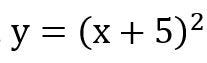
Now our goal is to find a value of x which will minimize the function, y ultimately makes it 0. We will define the steps to follow to attain our goal as follows,

Step 1: Start with random initial value of a variable, x=-3

Step 2: Calculate the gradient of the function by taking the first-order derivative of the function,

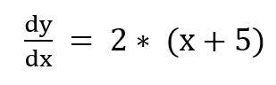
Step 3: Initialize the parameters, x = -3, learning rate = 0.01 (decides the factor of the gradient to obtain optimal value of x.

# Iteration 0
Find the value of y ,

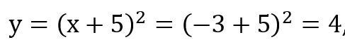
We will calculate the error,

E(y)= |expected value — calculated value| = |0–4| = 4

Now we will try to reduce this error through a set of iterations with updation of the value of x with respect to the gradient of a function.

# Iteration 1

With this new value of x, calculate the function,

Calculate the error,

E(y) = |expected value — calculated value| = |0–3.8416| = 3.8416

#Iteration 2

With this new value of x, calculate the function,

y=(x+5)²=(-3.0792+5)2=3.6894,

Calculate the error,

E(y)= |expected value — calculated value| = |0–3.6894| = 3.6894

Over the number of iterations, finally, we will achieve the global minima of the function, y=(x+5)² for x=-5, this process of continuous change in the value of x in proportion with negative of the gradient of the function is called as gradient descent algorithm.

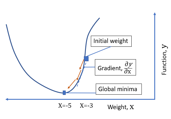
The diagram shows the process of optimizing the value of x to minimize the error function, E(y) to reach the global minima for the function, y. We started with random value of x and reached its optimal value to minimize the value of the function, y through a set of iterations through which we converged the value of x to its optima.

In the next section, we will take a look at how the artificial neural networks are evaluated and how their performance is measured with the different cost functions and evaluation metrics

Evaluating and Tuning the Artificial Neural Network

A neural network once trained on training data should be evaluated on test data to check its ability to predict unseen data. With the performance evaluation, we can judge the ability of a neural network to predict accurate results. Validation of the trained models should be done to assess its ability to generalize over a previously not seen data.

Firstly, we divide the dataset into three parts with some ratio, say 60:20:20 meaning that 60% data is reserved for model training, 20% for validating and fine-tuning the model, and 20% data will be used for testing a trained model. Validation data is a fraction of training data used for evaluating the model and accordingly fine-tune its performance using different hyperparameters.

Let’s define the three terminologies as follows

· Training Dataset is a subset of the dataset used to train a neural network; usually, a major fraction of a dataset is given for training purposes.

· Validation Dataset is a minor subset of data specifically used for validating the performance of the trained model and accordingly tune up the hyperparameters to control the learning of a model as per the requirements.

· Test Dataset is a fraction of the dataset used to test the performance of a trained model with different evaluation metrics such as precision-recall, F1 score, ROC, and AUC curves.

Major cost functions that are used for evaluating the performance of neural learning model are as follows,

· loss: It’s the cost measure to calculate loss function on training data

· val_loss: It’s the cost measure to calculate loss function on validation data

· acc: It’s a cost function to measure the accuracy of the learning model on training data.

· val_acc: It’s a cost function to measure the accuracy of the learning model on validation data

Now, let’s discuss some important scenarios with respect to loss and accuracy on training and validation data that need to be discussed.

If validation loss starts increasing with a decrease in loss of training data it shows that a learning model is overfitting on training data, and one should opt for different regularization techniques.

If a validation loss starts decreasing with an increase in validation accuracy, it shows that a learning model is getting generalized and possibly gives a good fit.

If a loss of training data starts decreasing without any increase in validation loss, we can continue the training on the model. But, as soon as validation loss starts increasing, it’s better to stop training a model further as it might lead to overfitting, as a result, a learning model will not get generalized well.

In the deep learning library, Keras, a set of evaluation metrics have been defined for regression analysis that is mean absolute error, root mean squared error, mean absolute percentage error, and cosine distance. While in case of classification problems, a list of measures like binary accuracy, categorical accuracy, top k categorical accuracy can be used.

Typically, metric scores are calculated at the end of each iteration or epoch for training data but if validation is also fed then metric scores are calculated for validation data as well, this will further help in tuning up a neural network with different regularization and optimization techniques.

Hyperparameters are vital to control the performance of the model. For a neural network, learning rate, number of epochs, number of hidden layers, number of hidden nodes, activation functions are major hyperparameters to be considered. Choosing the right parameter plays a significant role in the success of neural network architecture since it makes a major impact on the learning model.

Classical Machine Learning vs Deep Learning

Artificial intelligence is the ability of a machine to learn the different features of the data by itself and accordingly update the response with respect to that change in the characteristics of the data. Artificial intelligence is also known as machine intelligence meaning that the ability of a machine to perceive to its environment and accordingly generate the optimal response with the maximum success of getting the goal attained.

Artificial intelligence tries to mimic human intelligence by the way of experiential learning, in which it tries to correct its action based on the learning experience. Machine learning is the subset of artificial intelligence which builds a learning model based on the sample data, a set of known data points or observations, and their responses without explicitly defining the set of rules programmatically while deep learning is an advanced version of machine learning having strong capabilities of capturing non-linear complex relationships in the data.

Deep learning algorithms perform better with more amount of data while with machine learning algorithms, performance gets stagnant at a certain level regardless of the amount of data. In the case of deep learning algorithms, the data is a major constraint for better performance, the more the data, the higher will be the performance.

Deep learning algorithms require heavy computational resources for getting trained on large amounts of data while in the case of machine learning algorithms, commodity hardware can do the work. In machine learning, the domain expert has to identify the strong features for better predictability, but deep learning employs the stacked layer of neurons introducing non-linearity in its computation. Deep learning algorithms build a learning model with millions of parameters that hold a highly complex non-linear representation of the data.

Summary

In this post, we learned the transition of AI from classical machine learning to deep neural networks, starting with foundations of machine learning, supervised and unsupervised machine learning to multi-layered feed-forward neural networks along with different activation functions like a sigmoid, hyperbolic tangent, rectified linear unit and softmax. We learned the backpropagation algorithm and how it updates the weights or parameters of neural networks based on the gradient of the loss function. We studied about how to tune up a performance of a learning model with different hyperparameters like learning rate, number of hidden layers, number of nodes in hidden layers along with different cost functions.

---

Understanding Artificial Neural Networks — Perceptron to Multi-layered Feedforward Neural Network was originally published in Towards AI — Multidisciplinary Science Journal on Medium, where people are continuing the conversation by highlighting and responding to this story.

Published via Towards AI