The Architecture and Implementation of LeNet-5

Last Updated on January 6, 2023 by Editorial Team

Last Updated on July 30, 2020 by Editorial Team

Author(s): Vaibhav Khandelwal

Deep Learning

Demystifying the oldest Neural Network Architecture of LeNet-5

This very old neural network architecture was developed in 1998 by a French-American computer scientist Yann André LeCun, Leon Bottou, Yoshua Bengio, and Patrick Haffner. This architecture was developed for the recognition of handwritten and machine-printed characters. It is the basis of other deep learning models.

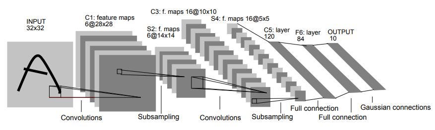
The architecture consists of a total of 7 layers consisting- 2 sets of Convolution layers and 2 sets of Average pooling layers which are followed by a flattening convolution layer. After that, we have 2 dense fully connected layers and finally a softmax classifier.

Input Layer

If we take a standard MNIST image for our understanding then we have an input of (32×32) grayscale image which passes through the first convolution layer with the 6 feature maps or filters having the size of (5×5) kernel and with a stride as 1. The values of the input pixels are normalized so that the white background and foreground black corresponds to -0.1 and 1.175 respectively, making mean approximately as 0 and the variance approximately as 1.

This input layer is not counted under network structure of LeNet-5 as traditionally, the input layer wasn’t considered as one of the network hierarchy.

First Layer

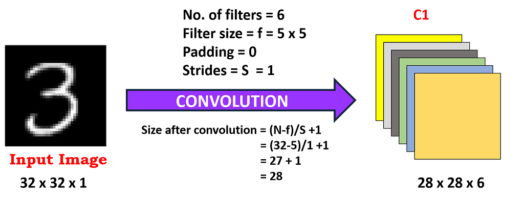
The result of the convolution of an input image with 6 filters has to lead to the change in dimension from (32x32x1) to (28x28x6) and we get our first layer. So, 1 channel is changed to 6 channels as 6 filters are applied to our input image. Also, the image size has been reduced as a result of zero paddings with a kernel size of (5×5).

> Calculations for the First Layer

• Filter size = f = 5 x 5
• No. of filters = 6
• Strides = S = 1
• Padding = P = 0
• Output featuremap size = 28 x 28
• No. of neurons = 28*28*6 = 4,704

In Convolution, filter values are trainable parameters.

• No. of learning parameters = (Weights + Bias )per filter * No. of filters

= (5 * 5 + 1) * 6 = 156

where, 5 * 5 = 25 are unit parameters and 1 bias per filter, and we have a total of 6 filters

• No. of connections = 156 * 28 * 28 = 1,22,304

> Detailed description:

1. The first convolution operation is applied on the input image (using 6 convolution kernels of size 5 x 5) to obtain 6 C1 feature maps (6 feature maps each of size 28 x 28), where size is obtained by (N-f+2P)/S+1, but as here P=0 and S=1, hence we are using N-f+1 throughout the content. Therefore, the output size after the convolution is 32–5 + 1 = 28.
2. Let’s take a look at the numbers of parameters that are needed. The size of the convolution kernel is 5 x 5, and there are 6 * (5 * 5 + 1) = 156 parameters in total, where +1 indicates that the kernel has a bias.
3. For the convolutional layer C1, each pixel in C1 is connected to 5 * 5 pixels and 1 bias, so there are 156 * 28 * 28 = 122304 connections in total. Though there are 1,22,304 connections, we only need 156 parameters to be learned, mainly through weight sharing.

Second Layer

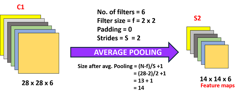
In the second layer, we implemented an average pooling layer with a filter size of (2×2) and a stride of 2. So, the resultant image dimension will decrease to (14x14x6). Here each unit in each feature map is connected to (2 x 2) neighborhood in the corresponding feature map in C1.

> Calculations for the Second Layer

• Filter size = f = 2 x 2
• No. of filters = 6
• Strides = S = 2
• Padding = P = 0
• Output feature map size = 14 x 14
• No. of neurons = 14*14*6 = 1,176

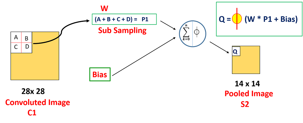
The 4 inputs are added to a unit in S2 from the corresponding feature map in C1 , then multiplied by a trainable coefficient, and added a trainable bias to it. The result is then passed through a sigmoidal activation function and we get the result Q

• No. of learning parameters = (Coefficient + Bias ) * No. of filters

= (1+ 1) * 6 = 12

where, the first 1 is the weight of the 2 x 2 receptive field corresponding to the pooling, and the second 1 is the bias.

• No. of connections = (2*2 + 1)*14*14*6 = 5,880

> Detailed description:

1. The pooling operation is followed immediately after the first convolution. Pooling is performed using 2 * 2 kernels, and 6 S2 feature maps of 14 * 14 are obtained.
2. The pooling layer of S2 is the average of the pixels in the 2 * 2 area in C1 multiplied by a weight coefficient plus an offset or bias, and then the result is mapped again.
3. So each pooling core has two training parameters, and thus in total there are 2*6 = 12 training parameters, but there are 5*14*14*6 = 5880 connections.

Third Layer

If we proceed further to the third layer, we are applying 16 filters with a kernel size of (5×5) to S2 resulting in a convolution layer C3 with 16 feature maps. This convolution results in changing the dimension of the image from (14 x 14 x 6) in S2 to (10 x 10 x 16) in C3.

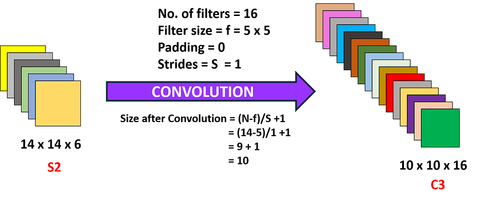
> Calculations for the Third Layer

• Filter size = f = 5 x 5
• No. of filters = 16
• Strides = S = 1
• Padding = P = 0
• Output feature map size = 10 x 10
• No. of neurons = 10*10*16 = 1,600

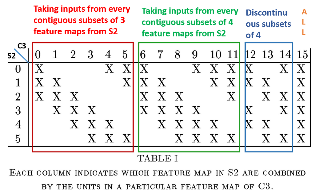
As here we can see that input i.e. S2 has 6 layers and the output i.e. C3 has 16 layers. Therefore we can not directly map each input layer to the output layer. So due to this, each unit in each feature map i.e. C3 is connected to several (5 x 5) neighborhoods at identical locations in a subset of S2’s feature maps.

The combination of different input feature maps selection from S2 will allow more new features to be extracted.

The different combinations of feature maps taken from S2 are shown in the figure below:

1. Taking inputs from every contiguous subset of 3 feature maps from S2:- First 6 convolution layers of C3 are made with this combination.
2. Taking inputs from every contiguous subset of 4 feature maps from S2:- Next 6 convolution layers of C3 are made with this combination.
3. Taking inputs from the discontinuous subset of 4 feature maps from S2:- Next 3 layers of C3 were made with this combination.
4. Taking all the feature maps:- The last layer of C3 is made with this combination.

• No. of learning parameters = (Parameters in combination type-1) + (Parameters in combination type-2) + (Parameters in combination type-3) + (Parameters in combination type-4)

= [6 * (5*5*3 + 1)] + [6 * (5*5*4 + 1)] + [3 * (5*5*4 + 1)] + [1 * (5*5*6 + 1)]

= 456 + 606 + 303 + 151 = 1516

NOTE:- In the above calculation the numbers 3, 4, 4, 6 used with 5*5 in the parenthesis are basically the depth.

• No. of connections = 1516 * (10*10)= 1,51,600

Fourth Layer

In the fourth layer, we’ll again apply the average pooling layer with the filter size as (2×2) and a stride of 2. So, the resultant image has a resultant of the average pool which will be of the dimension (5x5x16). Here each unit in each feature map of S4 is connected to (2 x 2) neighborhood in the corresponding feature map in C3.

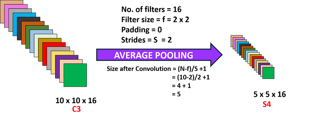
> Calculations for Fourth Layer

• Filter size = f = 2 x 2
• No. of filters = 16
• Strides = S = 2
• Padding = P = 0
• Output feature map size = 5 x 5
• No. of neurons = 5*5*16 = 400
• No. of learning parameters = (Coefficient + Bias ) * No. of filters

= (1+ 1) * 16 = 32

where, the first 1 is the weight of the 2 x 2 receptive field corresponding to the pooling, and the second 1 is the bias.

• No. of connections = (2*2 + 1)*5*5*16 = 2,000

This completes 2 convolution operations and 2 pooling operations.

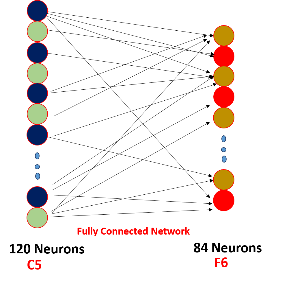
Fifth Layer

In the fifth layer, we have a fully connected Convolution layer C5 that has 120 neuron units, and each unit of C5 is connected to (5 x 5) neighborhood on all 16 of S4’s feature maps i.e. every unit of C5 is connected to all the feature maps of S4 and, thus C5 is known as Fully Connected Convolution Layer.

C5 is named as “Fully connected Convolution Layer” instead of simply “Fully connected layer” because if input size to the LeNet-5 is increased keeping everything else constant, the dimension of feature maps in C5 layer would be greater than (1 x 1).

So in the fourth layer, the resulting dimensions are (5x5x16), so the total nodes are 5x5x16 = 400 neurons. That means, 400 nodes are connected to 120 nodes as a dense fully connected network.

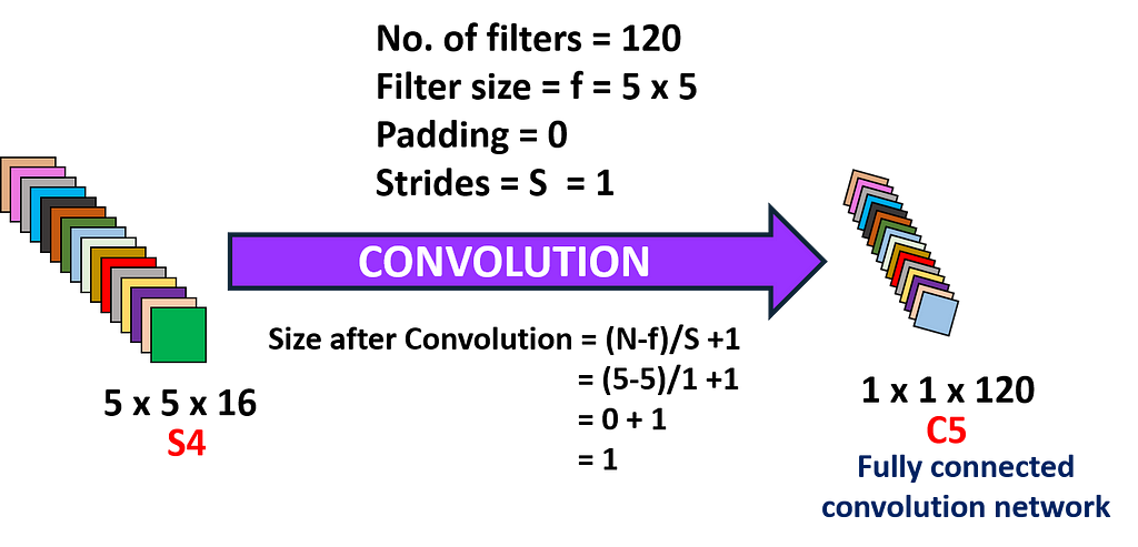
> Calculations for the Fifth Layer

• Filter size = f = 5 x 5
• No. of filters = 120
• Strides = S = 1
• Padding = P = 0
• Output feature map size = 1 x 1
• No. of neurons = 1*1*120 = 120
• No. of learning parameters = (5*5*16 + 1)*120 = 48,120
• No. of connections = 48,120*1*1 = 48,120

Sixth Layer

The Sixth layer F6 consists of 84 neurons Fully connected with C5. Here dot product between the input vector and weight vector is performed and then bias is added to it. The result is then passed through a sigmoidal activation function.

> Calculations for the Sixth Layer

• Input: C5 with 120 neurons
• Output: F6 with 84 neurons
• No. of learning parameters = (120*84) + 84 = 10,164

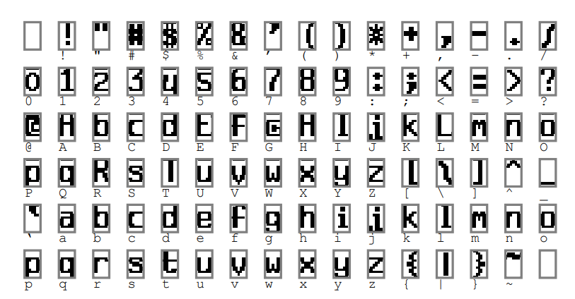
The number of neurons in the F6 layer is chosen as 84, corresponding to a 7 x 12 bitmap, -1 means white, 1 means black, so the black and white of the bitmap of each symbol corresponds to a code. Such a representation is useful for recognizing strings of characters taken from the printable ASCII set. The characters that look similar and confusing as Uppercase O, 0, and lowercase O will have the same output codes.

The ASCII encoding set is as follows:

And finally, we have a fully connected softmax output layer with 10 possible values corresponding to the digits from 0 to 9.

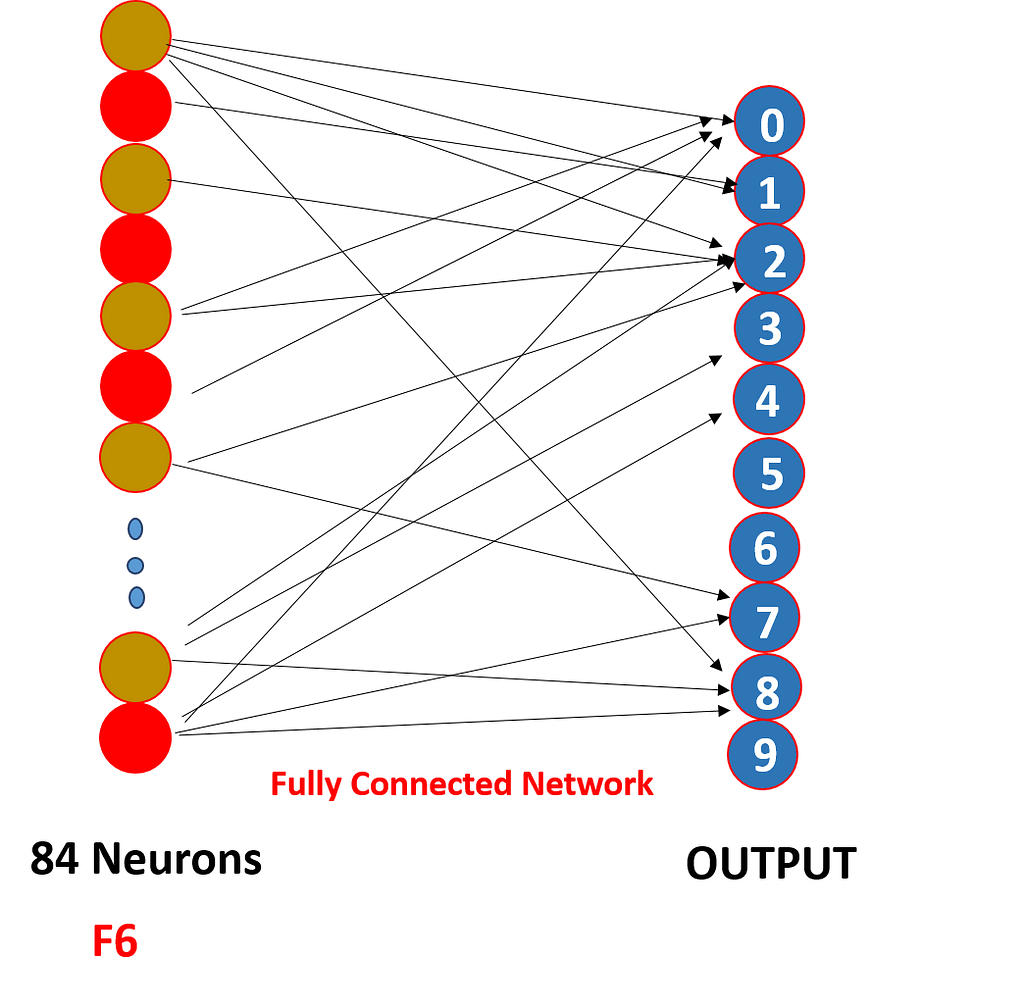
So we have “softmax activation” function on the output layer and other layers which we saw have “tanh” as the activation function as softmax will give the probability of occurance each output class at the end.

We are now venturing into coding territory.

Implementation of LeNet-5 using Keras

Before we start implementing the LeNet-5 through code, there are few key points to be kept in mind:

1. The input used by LeCun was of the size (32 x 32) but as we will be using the MNIST dataset, so the image size in this dataset is (28 x 28). Thus, the input size we’ll be having is (28 x 28).
2. When LeCun applied the third convolution i.e. C5, the input size was(5 x 5) but as from the initial only our input size to the network is less as compared to what LeCun took and hence, the input size for C5 in our case would be (4 x 4) and applying convolution to this input with (5 x 5) filter would result in a negative dimension size which is not possible and hence we’ll apply Flatten() after S4.

Importing Libraries

Loading the dataset and performing train-test split

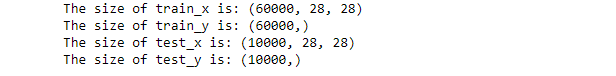
Checking the sizes of train and test split

The output of the above code will be as follows:

Performing reshaping operations- Converting into 4-D

Normalizing the values of the image- Converting in between 0 and 1

One-hot encoding the labels

Building the Model Architecture

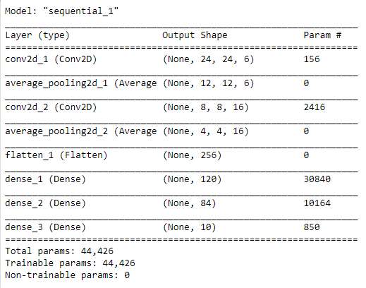
Summary of the model

• There are approx 45 thousand trainable parameters here as can be seen from the subsequent image.

Compilation of the model

And finally, a bit on evaluating your model.

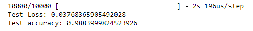
Finding the loss and accuracy of the model

The output of loss and accuracy is as follows:

📌 To get the complete code of LeNet-5 or any other network visit my GitHub repository.

References:

[1] Yann LeCun, Gradient-Based Learning Applied to Document Recognition(1998), Proc of the IEEE(1998)

Thanks for reading. Hope this blog would have helped you with both the coding and understanding of the architecture. 😃

---

The Architecture and Implementation of LeNet-5 was originally published in Towards AI — Multidisciplinary Science Journal on Medium, where people are continuing the conversation by highlighting and responding to this story.

Published via Towards AI