History of Neural Network! From Neurobiologists to Mathematicians.

Last Updated on July 30, 2020 by Editorial Team

Author(s): Ali Ghandi

Deep Learning

History of Neural Networks! From Neurobiologists to Mathematicians.

If you are familiar with Neural Networks and Deep learning, you might wonder what the relation between Neurons and the brain and these networks is. It seems they are based on some mathematical formulas and are far from what our brain does. You are right. It is math. Back in 1930, some scientists started to think about brain functionalities and tried to simulate neurons functionality as best as they could. They wanted a model that obeys all neurology rules and has the brain’s abilities.

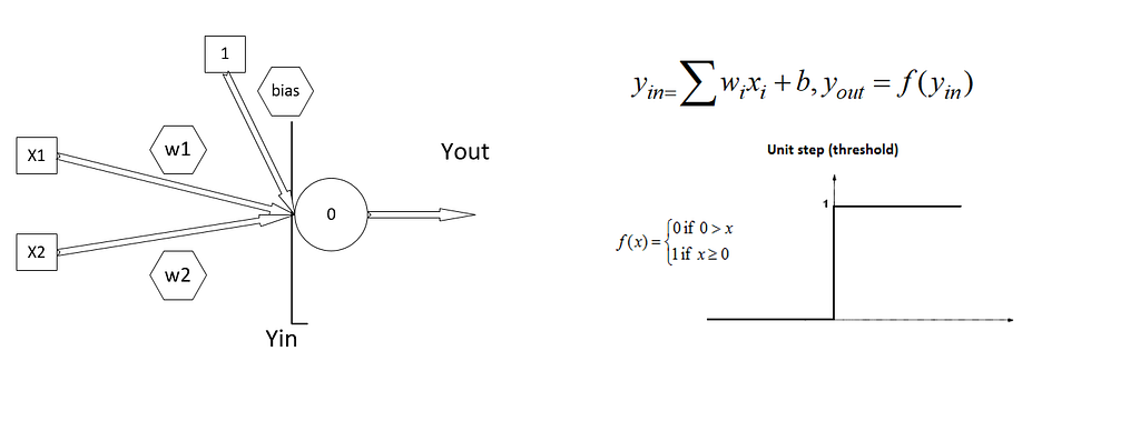
In 1943, McCulloch and Pitts made a computational unit by mimicking the functionality of a biological neuron. Their unit was so simple. It obeyed a threshold function. Neurons would fire a spike when their input signal passes a threshold. McCulloch and Pitts accumulated weighted inputs and gave it to this threshold function. The result was amazing! They built the first simulation of the brain, which could not learn, but as you set model weights, it can do some boolean algebra computations, like AND function.

In 1949, Hebb, a psychologist, tried to prove his theory about learning using McCulloch and Pitts’s neurons. He said that learning happens if an event occurs while it causes an output. In boolean algebra, it means learning of weights happens just in case both Input and output are True (or 1). True means something happens. Hebb rule is just a simple formula:

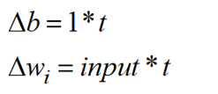
By these equations, a change in w only happens when both input and outputs are 1. One fundamental difference he made in McCulloch and Pitts’s model was turning threshold values to a bias weight. So he could simply learn this bias using the rule and leave threshold to fix number like one. In the case of AND function, the rule finds the right weights and makes a line that separates samples. The problem was that Hebb learned just in case both input and output are True, so it can not recognize samples that did not learn them at all. Here is a sample Hebb learning for AND function:

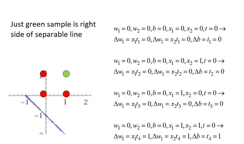
So w1=1 and w2=1 and bias=1 make a 2-d line which separates the feature space x1-x2 in 2d dimension. As you see, learning just happens when x1=1 and x2=1 and target(t)=1. That is the green point. Just it is on right side of out f function as f is defined as:

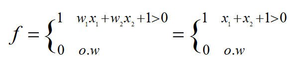
From the commutative property in sum, we can understand that the order of introducing patterns is not important.

But wait! We see the Hebb model does not learn when at least one of input or output is zero. So why do we insist on binary values? We can use bipolar(-1,1) instead, and now Hebb takes effect by -1 values too. So later in the 1950s, scientists extended Hebb rule to bipolar system. So Hebb became the first approved model that could learn partially of some boolean functions.

If you put some Hebb neurons next to each other, they can learn independently (which is a kind of weakness), and you will have a Hebb network. You can use a Hebb network for pattern recognition. If your pattern is linearly separable, each neuron makes a hyperplane to separate feature space, and you can learn your pattern. For example, the first neuron can separate alphabet A from others, and the second one separates alphabet B, and so on. You can imagine alphabet images have some overlay, and your Hebb network is too naive to do a good job on this, but it can learn, and you can check it.

Let’s do a pattern association from an image in 15*10 resolution to 7*9 one and reconstruct a character, so we have a comprehensive intuition about what modern Neural Network’s grandparents do.

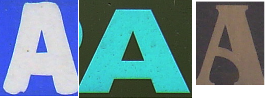
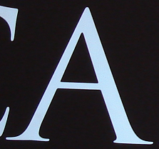
Imagine we have different fonts of A, and we resize them to have the same size. Let’s say the size is 15*10, so we have 150 inputs. Think of each pixel as an input. We want to just learn what A is and reconstruct its pattern. For example, we want to map these chars to a 7*9 image of A, which has less detail. We are doing pattern association. This means we assign some patterns to a special one. So we have 63 neurons each produce one pixel in output. Using Python, you can easily write the algorithm. You have 150 inputs and 150 weights, and you have three patterns to show your network (in AND function, we had four patterns to show). So you take three steps and update weights and done!

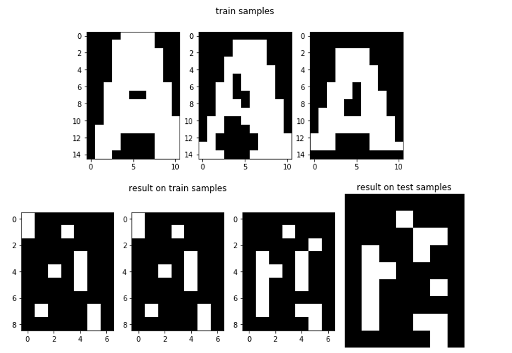
The first row is what we introduced to the Hebb network, and the second row is the response of the network to the same train data and one unseen data. As you see, Hebb just recognizes some parts of the character even on train data. It is a very simple network. However, it has the ability to learn part of this pattern association that assigns from 150 dimensions to 63 dimensions. You can extend neurons to recognize other characters too. If you make patterns simpler and reduce resolution, you will find amazing results. Some threshold functions independently learn what should be neurons output and reconstruct your pattern.

So as you see, we have a one-layer feed-forward network that is just a threshold function. From the boolean algebra world, we know we can simulate every function using the sum of the product (OR of some ANDs). It means that with some AND and OR functions, we can build any function in just two layers. And before we learn how to make AND, and OR boolean functions. So we need to make a two-layer network. But as Hebb says, the relation between input and output should be obvious to us. Adding a hidden layer and then we cannot understand the relationship between input and output. It seems that Hebb networks cannot exceed one layer. So we need something that tells us what the relation of the input of one layer with its output is. It means we should understand if an error happens in outputs, which input weights cause it, and how much.

So the next generation of NN started to appear in 1960 during world war. Americans tried to shoot Nazi ballistic rockets when they find new networks called Adaline.

In the next post, I say more about Adaline and how it changes thinking about NN. Adaline comes from the math world, not biology. So NN researchers, from here, became two groups. One that uses math to extend NN and second that enjoy simulating spiking neural networks and make biological models.

---

History of Neural Network!from neurobiologists to mathematicians. was originally published in Towards AI — Multidisciplinary Science Journal on Medium, where people are continuing the conversation by highlighting and responding to this story.

Published via Towards AI