Statistical Forecasting for Time Series Data Part 5: ARMA+GARCH model for Time Series Forecasting

Last Updated on January 6, 2023 by Editorial Team

Last Updated on December 26, 2020 by Editorial Team

Author(s): Yashveer Singh Sohi

Data Visualization

In these series of articles, the S&P 500 Market Index is analyzed using popular Statistical Model: SARIMA (Seasonal Autoregressive Integrated Moving Average), and GARCH (Generalized AutoRegressive Conditional Heteroskedasticity).

In the first part, the series was scrapped from the yfinance API in python. It was cleaned and used to derive the S&P 500 Returns (percent change in successive prices) and Volatility (magnitude of returns). In the second part, a number of time series exploration techniques were used to derive insights from the data about characteristics like trend, seasonality, stationarity, etc. With these insights, in the 3rd and 4th part the SARIMA and GARCH class of models were explored. The Links to all these parts are at the bottom of this article.

In this part, the 2 models introduced previously (SARIMA and GARCH) are combined to build predictions and effective confidence intervals for S&P 500 Returns. The code used in this article is from Returns Models/ARMA-GARCH for SPX Returns.ipynb notebook in this repository

Table of Contents

1. Importing Data
2. Train-Test Split
3. Parameter Estimation for ARMA
4. Fitting ARMA Model on Returns
5. ARMA Model Residuals
6. GARCH Parameter Estimation
7. GARCH Model on ARMA Residuals
8. Predictions of ARMA + GARCH model
9. Conclusions
10. Links to other parts of this series
11. References

Importing Data

Here we import the dataset that was scrapped and preprocessed in part 1 of this series. Refer part 1 to get the data ready (linked at the end), or download the data.csv file from this repository.

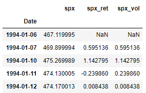
Since this is same code used in the previous parts of this series, the individual lines are not explained in detail here for brevity.

Train-Test Split

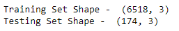
We now split the data into train and test sets. Here all the observations on and from 2019–01–01 form the test set, and all the observations before that is the train set.

Parameter Estimation for ARMA Model

ARMA model is a subset of the ARIMA model, discussed previously in this series. It has 2 parameters represented as: ARMA(p, q). Like ARIMA,

• The number of significant lags in PACF plot indicates the order of p (which controls the effect of past values on present value).
• The number of significant lags in the ACF plot indicates the order of q ( which controls the effect of past residuals on the current value).

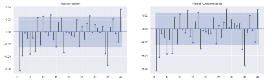
The plot_acf() and plot_pacf() functions from the statsmodels.graphics.tsaplots library are used to plot the ACF and PACF plots for S&P 500 Returns. On examining the plots, it is clear that the first 2 lags are significant in both the plots. After these, the significance level shuts off abruptly and then spikes up again. Thus, to keep the model simple, it is reasonable to set the initial parameters as:

• p = 1, or p = 2
• q = 1, or q = 2

Fitting ARMA Model on Returns

Let’s build the ARMA(1, 1) model on S&P 500 Returns.

Note: Before Fitting a model from the SARIMA class of models, one needs to check whether the input series used to fit the model is stationary. For a stationary time series the summary statistics do not change significantly over time. This means that the underlying process creating the data is the same as time passes on. It is intuitive to expect that one can only model a series if the underlying process generating the series remain the same in the future. The stationarity of this series spx_ret is tested in previous parts (part2 and part3) of this series using the adfuller() test from statsmodels.tsa.stattools .

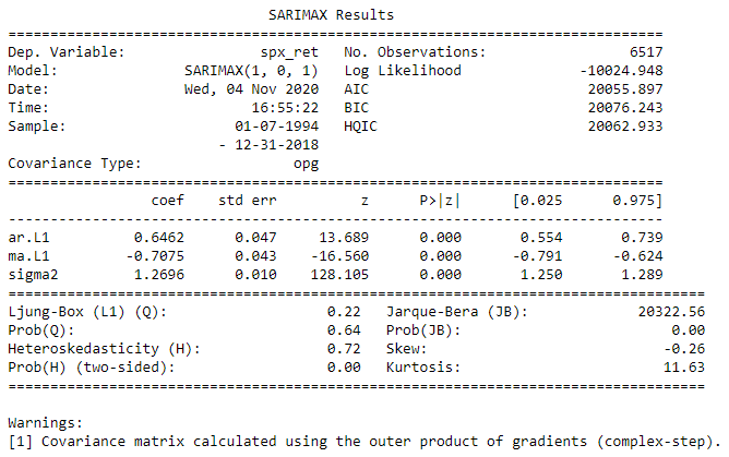
The SARIMAX() function in the statsmodels.tsa.statespace.sarimax library is used to fit any subset of the SARIMAX family of models. The series, spx_ret , and the order, order = (1, 0, 1) , are passed in the function to get the ARMA(1, 1) model definition. The fit() method on the model is used to train the model definition. The summary() method on the fitted model results prints the summary table of the model as shown the image.

The summary table shows that all the coefficients of the model are significant.

ARMA Model Predictions and Confidence Intervals

In this section we use the ARMA(1, 1) model to forecast the Returns for the Test set. Furthermore, the same model is used to generate the confidence intervals.

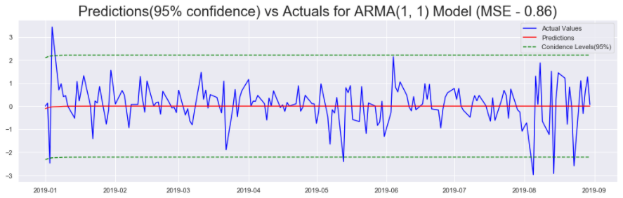
The get_forecast() method is used to build a forecasts object that can later be used to derive the confidence intervals using the conf_int() function. The predict() function is used to get the predictions for the test set. The RMSE (Root Mean Squared Error) metric is used to calculate the accuracy of the predictions with respect to the actual returns in the test set. The predictions and the confidence intervals are then plotted against the actual returns from the test set to visually confirm the accuracy of the model.

On inspecting the plot (shown in the image), the predictions are in some cases spot on, and in some cases they are wrong by huge margins. The confidence intervals do nothing to indicate how the predictions will perform in different time periods of the test set. In some cases the confidence intervals seem too conservative, and the returns overshoot the boundaries. In other cases, the confidence intervals are not nearly conservative enough.

To address this issue, in the next section we will analyse the residuals of the model and try to predict when the ARMA predictions will be off by a small margin and when will they be off by a large margin.

ARMA Model Residuals

In this section we plot the residuals of the model and explore some of its properties.

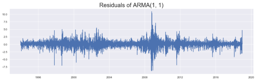
The residuals generated by the ARMA(1, 1) model can be accessed by using the resid attribute of the fitted model. On examining the plot, it is clear that the residuals show the phenomenon of volatility clustering. This means that if the series shows high volatility (high variance) at a particular time step, then it will show high volatility in nearby time steps as well, and vice versa. In periods around 2004, 2008 (periods of high volatility), and the periods in between(periods of low volatility), this phenomenon is clearly observed.

Series that show such volatility clustering can be successfully modeled using the GARCH model(as seen in part 4 linked at the end). In the next section we start estimating the parameters needed to fit the GARCH model on the residuals of ARMA(1, 1) model.

GARCH Parameter Estimation

The GARCH model, has 2 parameters represented as: GARCH(p, q). These parameters are estimated by counting the number of significant lags in the PACF plot. The code to generate such a plot is not shown as it is very similar to the PACF plot code above. Only tweaks needed are in the data passed. In this case the series passed will be model_results.resid .

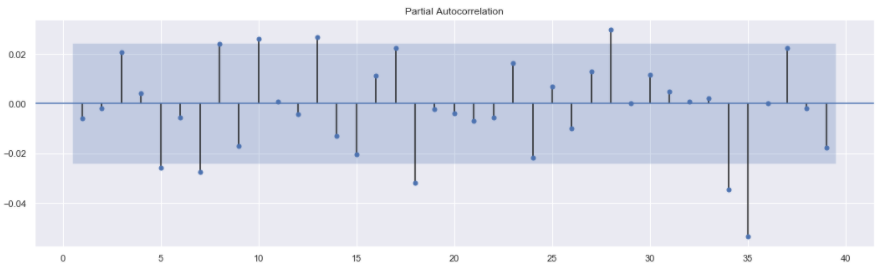
The plot shows that there are no significant lags in the residuals. Thus we will fit various GARCH models: GARCH(1, 1), GARCH(1, 2), GARCH(2, 1), GARCH(2, 2), etc. till we get a model with significant coefficients and best accuracy.

GARCH Model on ARMA Residuals

As mentioned in the previous section, the PACF plot did not offer any insight for starting parameters. In such case, various models should be fit in order to find one that has significant coefficients and best accuracy. This ensures that we have the simplest possible model with the best possible accuracy.

After fitting a few such model, the GARCH(2, 2) satisfied this criteria in my case. Feel free to try out various models locally and choose your preferred model. Let us see the code to fit the GARCH(2, 2) model:

Before fitting the model, a new dataframe is prepared. This dataframe consists of all the time steps in the original dataset (before train-test split). The training time steps are occupied by the Residuals from the ARMA(1, 1) model. These are actually used for training the GARCH model. The testing periods are occupied by the actual returns observed one time step previously. This is tantamount to saying that the model will forecast tomorrow’s volatility in returns using the returns observed today.

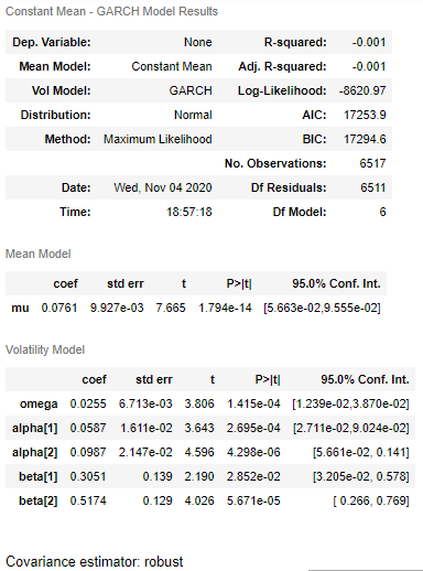
The arch_model() function in arch library is used to define a GARCH model. The fit() function is used to train the model defined. The last_obs argument is used to identify from what time step should the model start predicting. The summary() function prints out the summary table as shown in the image. The summary table shows all coefficients of the model are significant.

Predictions of ARMA+GARCH model

In this section we use the GARCH(2, 2) model fitted on residuals of ARMA(1, 1) to predict the volatility of the residuals in the test set.

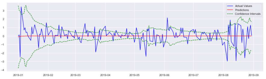
The forecast() method is used on the fitted model: resid_model_results . This outputs an ARCHModelForecast object that contains the predictions for the mean model, and the volatility model. Next, the residual_variance attribute is called to get the predictions for volatility. The predictions from the volatility model are subtracted (and added) to the predictions from the ARMA model stored in the arma_predictions_df to get the lower (and upper) confidence interval(s) of the model.

Next, the predictions (from ARMA(1, 1)) and the confidence intervals (from GARCH(2, 2)) are plotted against the actual S&P 500 Returns. On examining the plot, it is clear that when the returns are stable, and when the predictions are close to actual returns, the confidence intervals reflect this by being close. Same is true for when the Returns are unstable and the predictions are far from the Returns. In this case too the confidence intervals adjust and become far apart.

Conclusions

Thus, using the combination of ARMA and GARCH models we are able to build much more meaningful forecasts. Looking at the forecasts and confidence intervals we can understand the ballpark figure for future returns and also the stability in the market. In the next and final article in this series, we will look at how to use the SARIMA family of model for Non-Stationary data: S&P 500 Prices.

Links to other parts of this series

• Statistical Modeling of Time Series Data Part 1: Preprocessing
• Statistical Modeling of Time Series Data Part 2: Exploratory Data Analysis
• Statistical Modeling of Time Series Data Part 3: Forecasting Stationary Time Series using SARIMA
• Statistical Modeling of Time Series Data Part 4: Forecasting Volatility using GARCH
• Statistical Modeling of Time Series Data Part 5: ARMA+GARCH model for Time Series Forecasting.
• Statistical Modeling of Time Series Data Part 6: Forecasting Non — Stationary Time Series using ARMA

References

[1] 365DataScience Course on Time Series Analysis

[2] machinelearningmastery blogs on Time Series Analysis

[3] Wikipedia article on GARCH

[4] ritvikmath YouTube videos on the GARCH Model.

[5] Tamara Louie: Applying Statistical Modeling & Machine Learning to Perform Time-Series Forecasting

[6] Forecasting: Principles and Practice by Rob J Hyndman and George Athanasopoulos

---

Statistical Forecasting for Time Series Data Part 5: ARMA+GARCH model for Time Series Forecasting was originally published in Towards AI on Medium, where people are continuing the conversation by highlighting and responding to this story.

Published via Towards AI