In Homage to Benoit Mandelbrot

Last Updated on December 23, 2020 by Editorial Team

Author(s): Jonathan Scott

Brownian Motion in Multifractal Time

I must thank my good friend Daniel Luftspring for his contributions and guidance throughout the development of this project.

Short on the Assessment of Risk

At the core of the financial market theory, there is a large and unstable assumption. The assumption is that the risk of a financial instrument can be determined by its volatility and that this measure scales with the square root of time. To understand the origins of this assumption, you must travel back before the subprime mortgage crisis of 2008, the dot-com bubble of 2000, Black Monday in 1987, the Wall Street Crash of 1929, and then another one hundred years. Here, you will find Robert Brown looking through a microscope at a speck of pollen suspended in water. He observed that the speck danced erratically. In 1900, this observation was applied to finance with advanced mathematics by Louis Bachelier in his dissertation, Théorie de la spéculation, on modeling the stock market. With the assumption that the price of a stock moved in the same random manner as the speck of pollen, he was able to calculate a price for the stock’s option. In 1905, Albert Einstein studied the same process and provided a way to mathematically describe the movement of the particle. Einstein proved that the movement was attributed to the individual water molecules bombarding the speck of pollen. Additionally, he provided mathematics to show that the distance the speck travels from its origin scales at the square root of the time that has elapsed. In honor of Robert Brown, a process which moves in a statistically similar way to the speck of pollen is called Brownian motion.

To this day, financial market theory is based on the work provided by Bachelier and Einstein in the early 1900s. The distance the speck of pollen travels is comparable to the volatility of a financial asset, wherein the price range from the minimal value to the maximum value of a mean adjusted cumulative deviation series within a given length of time should scale with the square root of the length of that time period. In other words, the longer the time period, the larger the expected price range. A proper assessment of risk is necessary, as it is the basis for valuing financial assets and constructing efficient portfolios.

A Brownian motion’s movement is described by a Standard Normal Distribution. This famous distribution conveniently describes many complex systems. Therefore, it is understandable that Bachelier would assume the stock market could be described by this distribution. This is, however, a misclassification. Einstein proved the distance a Brownian motion process travels from its origin scales at the square root of time; however, it is commonly shown that a stock market’s variability will scale faster than the square root of time. Edgar E. Peters provides excellent empirical evidence of the true scaling rate in Fractal Market Analysis. This is to say that the market is more volatile than a Brownian motion suggests. Volatility has long been considered the essence of risk, and without a proper assessment of risk, financial instruments cannot be valued properly and investors will be blindsided by ruinous events in the market.

It is much like a theory of sea waves that forbids their swells to exceed six feet.
– Mandelbrot, Benoit. How Fractals Can Explain What’s Wrong with Wall Street.

Benoit B. Mandelbrot

Benoit Mandelbrot recognized the flaws of financial market theory models and attempted to provide an alternative — one which more accurately assessed risk. The model would generate a realistic time series with large swings in price and clusters of volatility. These were not accounted for by existing models.

Mandelbrot’s contributions to the mathematical community are vast and impactful, but perhaps his most notable contribution is his work on fractal geometry. A fractal, which is more formally described in the next sections, has a common characteristic: the structure is random locally and deterministic globally. Edgar E. Peters provides the example in Fractal Market Analysis of mammalian lung bronchi. The branching of bronchi at a microscopic level is random, but the global structure of the lungs is almost always deterministic. Similarly, the micro-movements of a stock appear random within short spans of time, but there is a more deterministic structure globally. Mandelbrot believed a simple fractal shape could explain the complex structure of the market. With apologies to him and his colleagues, this article attempts to describe his greatest method for emulating a financial market: Brownian Motion in Multifractal Time.

A Fractured Market

A fractal is a geometric shape that can be separated into parts, each of which is a reduced-scale version of the whole.
– Mandelbrot, Benoit. Scaling in Financial Prices: III. Cartoon Brownian motions in multifractal time.

Upon observing that the market looks similar at all scales, he was confident that a proper fractal could simulate the market and capture its key attributes: large swings and clustered volatility.

Fractal Price Generator

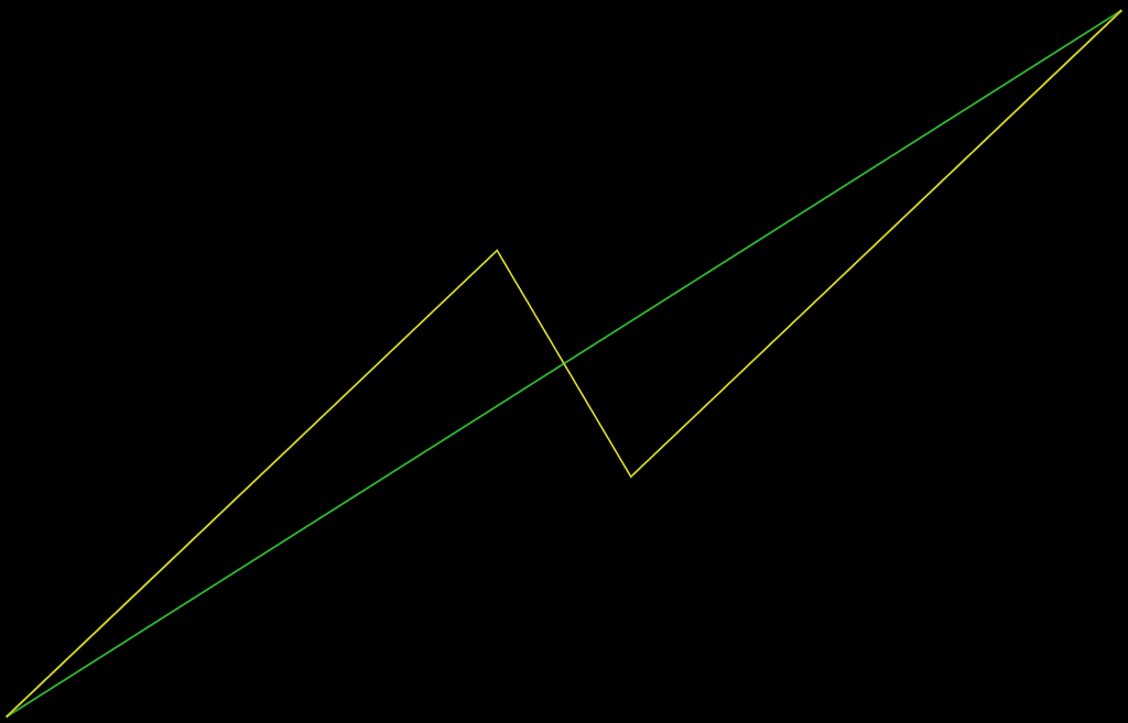
The root of a fractal is an initiator and a generator. In the case of Mandelbrot’s financial fractal, which is represented in Figure 1, the initiator is a straight line representing the price change, and the generator is a lightning bolt shape with two turning points and proceeds in an up-down-up fashion. The up-down-up procession allows for the up and down periods in the market. Each of the three straight line segments of the generator becomes the next iteration of initiators. Through infinite iteration, the fractal builds. Figure 2 iterates this process four times.

The model can be extended by randomizing each of the three segments of the generator as shown in Figure 3.

There is special generator for a Brownian motion process — the process from which financial theory builds. It is symmetric with the first turning point at y=2/3 and x=4/9. Iterate the Brownian motion generator such that each of the three segments is the same proportional width and height and the process will always be Brownian motion. Iterating the Brownian motion generator creates a visually realistic picture of the market, as seen in Figure 4.

This is a pretty picture which may pass a visual test, but the statistical properties of the Brownian motion generator are starkly different than that of a true market. It is often easier to look at the price differences between moments than the price chart when determining the fitness of the model. For example, Figure 4 passes the visual test of what a market’s price chart looks like, but it is visually clear that its moment to moment price changes, as represented in Figure 5, do not represent that of a true market (see Figure 6). The moment to moment price changes of the Brownian motion, represented in Figure 5, spread uniformly throughout time and the amplitude of very few changes fall out of the norm.

A true market’s moment to moment price changes will look like Figure 6. This figure displays clusters of volatility, unlike the uniform volatility in Figure 5. In Figure 6 it is more likely for a large change to be followed by more large changes, and for a small change to be followed by more small changes. Mandelbrot calls this long term dependence. Long term dependence is found in a true market and not within a Brownian Motion modeled market.

However, the Brownian motion generator can be altered to produce a realistic chart like Figure 6. This will be discussed in the following section.

Brownian Motion in Multifractal Time

Mandelbrot showed that fractals are versatile enough to accurately emulate the Brownian motion market, which is the basis of financial market theory. He adapts the Brownian motion, which is considered unifractal, to be a multifractal price generator, as described below. Such an adaptation is required to produce the large swings and clusters of volatility.

Multifractal Price Generator

It is commonly assumed that there are faster and slower periods of market activity. The Brownian motion generator can be altered to account for these fast and slow periods of time, which Mandelbrot states is the essence of volatility.

Each stage of the iteration starts with a Brownian motion generator (unifractal), and then contracts or lengthens each segment, as shown in Figure 7, in a prescribed way. The resulting generator is considered to be multifractal. The price (y coordinate) of the turning points remains the same, but the time (x coordinate) taken to reach that price changes. Since market activity is represented by the change in y, Figure 7 shows that the same amount of market activity occurs in a shorter amount of time for segments one and three, and a longer amount of time in segment two.

Figure 8 displays that the moment to moment price change chart of a multifractal generator has large swings and clusters of volatility.

The question arises, in what prescribed way should the Brownian motion unifractal price generator be altered so that it becomes multifractal and produces a realistic time series?

Clock Time vs Trading Time

Clock Time can be represented as a straight line — it progresses at the same rate, always. Markets, however, observe fast and slow periods of time, as though they follow some derivative of Clock Time. Mandelbrot coins this process Trading Time, and Trading Time does not progress linearly. Figure 9 displays Clock Time (straight line) transforming into Trading Time.

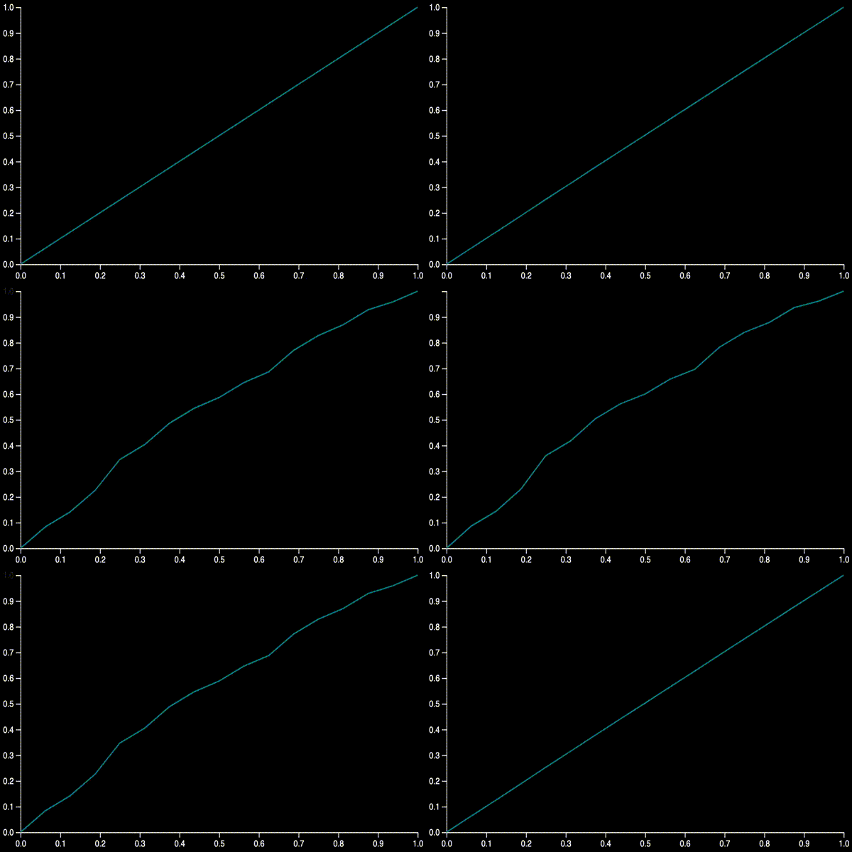
Mandelbrot believes that Trading Time progresses in a multifractal manner. The binomial multiplicative cascade, which is described below, is used to transform Clock Time into Trading Time, as it is known to be multifractal.

The binomial multiplicative cascade is a fractal. The initiator is a horizontal line, and the generator is a step function placed upon that horizontal line. To create the cascade, start by representing Clock Time as the initiator and define two weights that sum to one. For every initiator of Clock Time, bifurcate that initiator and allocate weight 1 to the area under the first half and weight 2 to the area under the second half. The total area under the initiator is maintained as the total area under the generator. One iteration of this process is shown in Figure 10.

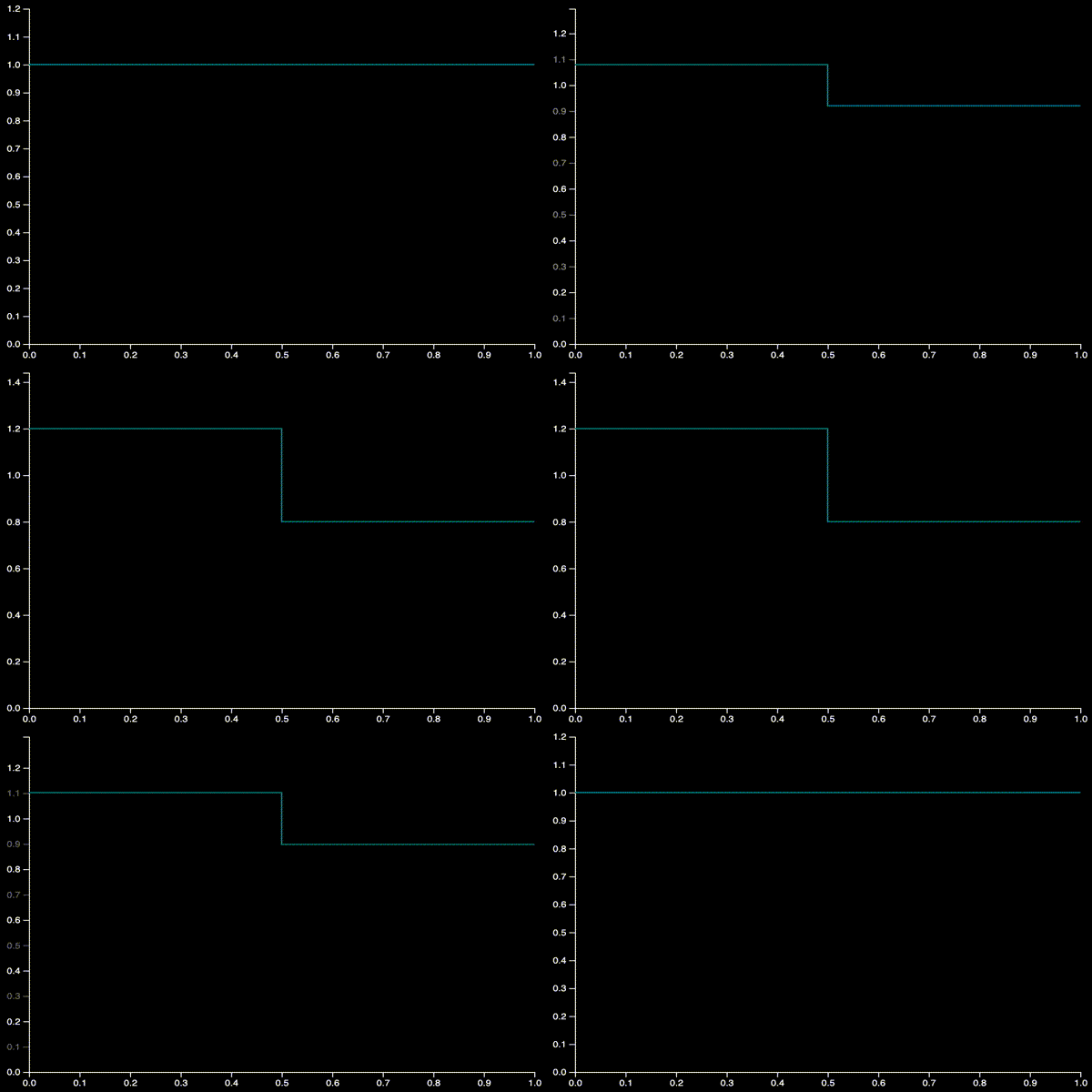
In the Figure 10, the area under the initiator is base x height = area, or 1 x 1 = 1. Weight 1 is selected as 0.6 and weight 2 as 0.4. After one iteration, weight 1 of the total area under the initiator is assigned to the first half of the generator. Likewise, weight 2 of the total area under the initiator is assigned to the second half of the generator. This produces two rectangles with width 0.5 and an unknown height. The equation for the first rectangle is 0.5 x height = 0.6, since bifurcating the initiator provides a known base and weight 1 determines that the area of rectangle 1 is 0.6. Solving for height produces 1.2. The same process is applied for rectangle 2. The area of 1 under the original initiator is maintained and calculated as the cumulative area of the generator’s two rectangles: (1.2 x 0.5) + (0.8 x 0.5) = 1. Figure 11 iterates the process four times.

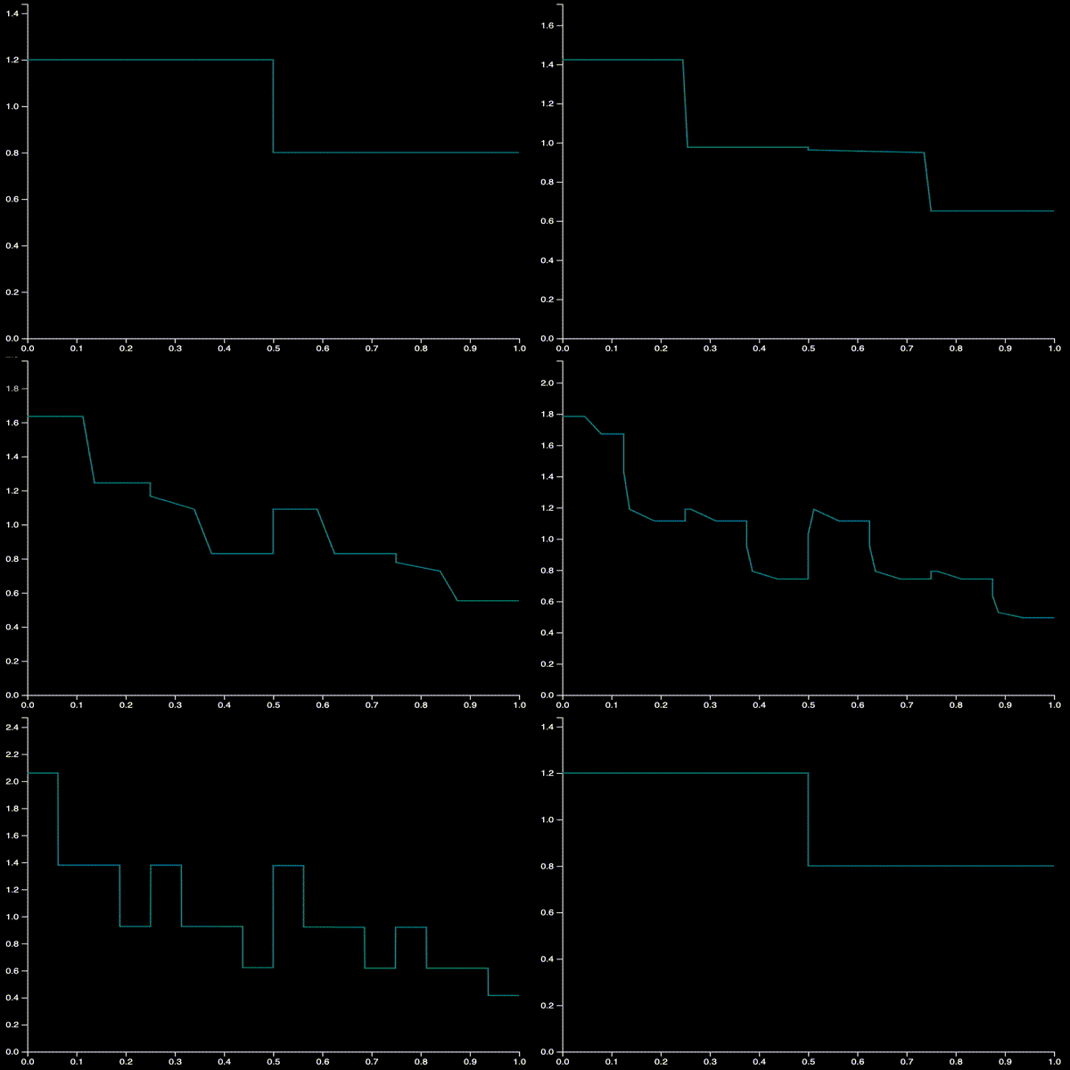
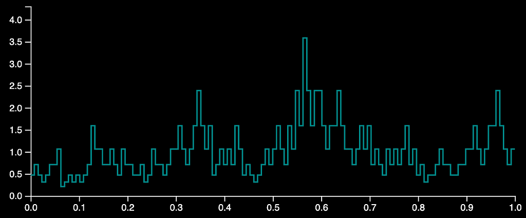
Randomizing the allocation of weights at each stage of the iteration and iterating many times produces the multiplicative cascade. As described above, the total area under the multiplicative cascade is equivalent to the total area under the original initiator. Therefore, the multiplicative cascade is a Probability Density Function (“PDF”) by construction. An example is shown in Figure 12.

The last step of converting Clock Time to Trading Time is to calculate the Cumulative Density Function (“CDF”) of the multiplicative cascade PDF. Figure 13 shows the Trading Time CDF.

Trading Time’s Effect on Brownian Motion

Trading Time transforms the Brownian motion generator into a multifractal price generator. The process is best illustrated in Figure 14 with three graphs: the Brownian motion generator, Trading Time, and the resulting multifractal generator.

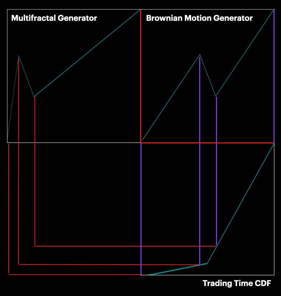
Figure 14 visualizes the transformation of the turning points of a Brownian motion generator (unifractal) into new turning points of the Brownian Motion in Multifractal Time generator (multifractal). Figure 14 is read from the turning points of the Brownian motion generator in the upper right quadrant, down to the Trading Time CDF in the lower right quadrant, and then over to the left and up to the new turning points of the multifractal generator. As shown in Figure 14, the Trading Time CDF is evaluated at each turning point of the Brownian motion generator. The difference in height between sequential turning points when projected onto the CDF (purple lines), becomes the width (red lines) of the corresponding multifractal generator segment. After the transformation, the width of each of the three segments of the Brownian motion generator has been altered by Trading Time. This alteration changes the length of time in which each segment’s market activity occurs. Since Trading Time is multifractal, the resulting generator is a Brownian motion that progresses in Multifractal Time.

Note:
I am hard pressed to find information that describes the exact process which ensures the new sum of the width values generated by the CDF maintain the sum of width values of the Brownian motion generator. I chose to follow this process.

Figure 14 is exaggerated for effect, and the CDF is only constructed with one iteration. In reality, the CDF is fully formed through many iterations of the binomial cascade before the first iteration through the fractal price generator. At each iteration of the fractal price generator, the CDF is evaluated to adjust the x coordinates of each turning point of the fractal price generator. This process transforms the unifractal price generator into a multifractal price generator. The resulting time series contains both large swings and clusters of volatility as shown in Figure 15 and Figure 16.

Figures 15 and 16 complete Benoit Mandelbrot’s Brownian Motion in Multifractal Time model. This model explains the complex structure of the market better than common financial market theory, and consequently provides a better assessment of market risk.

Concluding Remarks

The information provided in this article is a summary of Brownian Motion in Multifractal Time. It attempts to explain concepts from Mandelbrot’s publications in a simplified way. For more information about Brownian Motion in Multifractal Time, I encourage you to visit four sources which formed my knowledge base for this article:

• A Multifractal Model of Asset Returns. Benoit Mandelbrot. 1997.
• Scaling in Financial Prices: III. Cartoon Brownian motions in multifractal time. Benoit Mandelbrot. 2001.
• Surrogates of the Stock Market resource from Yale.
• The (mis)behaviour of markets: a fractal view of risk, ruin, and reward. Benoit Mandelbrot. 2004.

To construct a time series, visit this interactive site. If you are interested in the code which generates these time series, install the python package fractalmarkets and follow instructions on Github.

---

In Homage to Benoit Mandelbrot was originally published in Towards AI on Medium, where people are continuing the conversation by highlighting and responding to this story.

Published via Towards AI