Pandas Complete Tutorial for Data Science in 2022

Author(s): Noro Chalise

 

Originally published on Towards AI the World’s Leading AI and Technology News and Media Company. If you are building an AI-related product or service, we invite you to consider becoming an AI sponsor. At Towards AI, we help scale AI and technology startups. Let us help you unleash your technology to the masses.

Pandas Beginner to Advanced Guide

Pandas is one of the most popular python frameworks among data scientists, data analytics to machine learning engineers. This framework is an essential tool for data loading, preprocessing, and analysis.

Before learning Pandas, you must understand what is data frame? Data Frame is a two-dimensional data structure, like a 2d array, or similar to the table with rows and columns.

For this article, I am using my dummy online store data set, which is located in my Kaggle account and GitHub. You can download it from both. Also, I will provide you with all this exercise notebook on my GitHub account, so feel free to use it.

Before starting the article, here are the topics we covered.

Table of content

1. Setup
2. Loading Different Data Formats
3. Data Preprocessing
4. Memory Management
5. Data Analysis
6. Data Visualization
7. Final Thought
8. Reference

Feel free to check out GitHub repo for this tutorial.

1. Setup

Import

Before moving on to learn pandas first we need to install them and import them. If you install Anaconda distributions on your local machine or using Google Colab then pandas will already be available there, otherwise, you follow this installation process from pandas official’s website.

# Importing libraries
import numpy as np
import pandas as pd

Setting Display Option

Default setting of pandas display option there is a limitation of columns and rows displays. When we need to show more rows or columns then we can use set_option() the function to display a large number of rows or columns. For this function, we can set any number of rows and columns values.

# we can set numbers for how many rows and columns will be displayed
pd.set_option('display.min_rows', 10) #default will be 10 
pd.set_option('display.max_columns', 20)

2. Loading Different Data Formats Into a Pandas Data Frame

Pandas is an easy tool for reading and writing different types of files format. Using these tools we can load CSV, Excel, Pdf, JSON, HTML, HDF5, SQL, Google BigQuery, etc file easily.

Here are some methods, I will show you how we can read and write most frequently using file format.

Reading CSV file

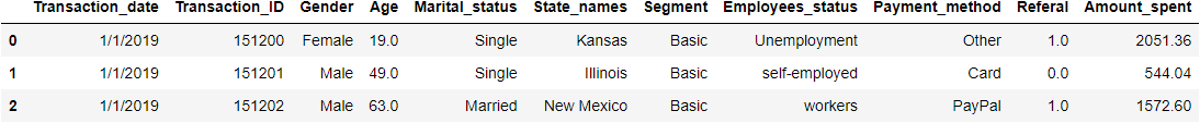
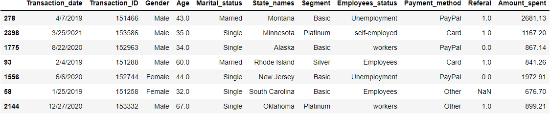
CSV (comma separated file) is the most popular file format. Reading this file we used the simply read.csv() function.

# read csv file

df = pd.read_csv('dataset/online_store_customer_data.csv')
df.head(3)

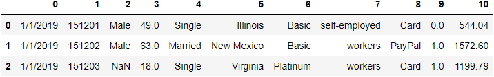
We can add some common parameters to tweak this function. If we need to skip some first rows in the data frame then we can use skiprows a keyword argument. For example, If we want to skip the first rows then we use skiprows=2. Similarly, if we don’t want to last 2 rows then we can simply use skipfooter=2 . If we don’t want to load the column header then we can use header=None .

# Loading csv file with skip first 2 rows without header
df_csv = pd.read_csv('dataset/online_store_customer_data.csv', skiprows=2, header=None)
df_csv.head(3)

Read CSV file from URL

For reading the CSV file form URL, you can directly pass the link.

# Read csv file from url
url="https://raw.githubusercontent.com/norochalise/pandas-tutorial-article-2022/main/dataset/online_store_customer_data.csv"
df_url = pd.read_csv(url)
df_url.head(3)

Write CSV file

When you want to save a data frame on a CSV file you can simply use to.csv() the function. You also need to pass the file name and it will save that file.

# saving df_url dataframe to csv file
df_url.to_csv('dataset/csv_from_url.csv')
df_url.to_csv('dataset/demo_text.txt')

Read text file

Reading a plain text file, we can use read_csv() the function. In this function, you need to pass the .txt file name.

# read plain text file
df_txt = pd.read_csv("dataset/demo_text.txt")

Read Excel file

To read an Excel file, we should use read_excel() the function of the pandas package. If we have had multiple sheet names then we can pass the sheet name argument with this function.

# read excel file
df_excel = pd.read_excel('dataset/excel_file.xlsx', sheet_name='Sheet1')
df_excel

Write Excel file

We can save our data frame to an excel file same as a CSV file. You can use to_excel() function with file name and location.

# save dataframe to the excel file
df_url.to_csv('demo.xlsx')

3. Data preprocessing

Data preprocessing is the process of making raw data to clean data. This is the most crucial part of data science. In this section, we will explore data first then we remove unwanted columns, remove duplicates, handle missing data, etc. After this step, we get clean data from raw data.

3.1 Data Exploring

Retrieving rows from a data frame.

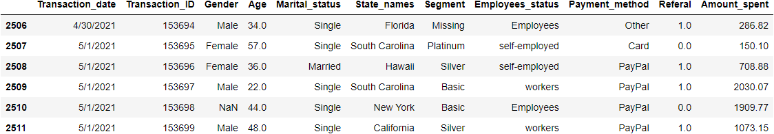
After the loading data, the first thing we did to look at our data. For this purpose we use head() and tail() function. The head function will display the first rows and the tail will be the last rows. By default, it shows 5 rows. Suppose we want to display the first 3 rows and the last 6 rows. We can do it this way.

# display first 3 rows
df.head(3)

# display last 6 rows
df.tail(6)

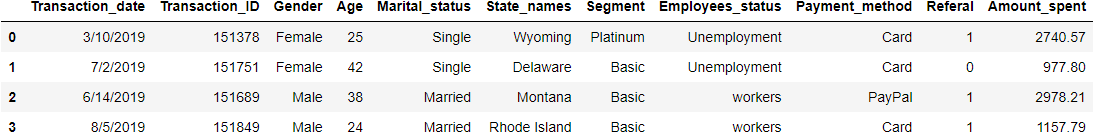
Retrieving sample rows from a data frame.

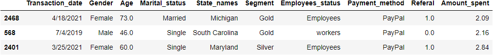
If we want to display sample data then we can use sample() a function with the desired number of rows. It will show the desired number of random rows. If we want to take 7 samples we need to pass 7 in the sample(7) function.

# Display random 7 sample rows
df.sample(7)

Retrieving information about the data frame

To display data frames information we can use info() the method. It will display columns data types, counting each column’s total non-null values and its memory space.

df.info()

<class 'pandas.core.frame.DataFrame'>
RangeIndex: 2512 entries, 0 to 2511
Data columns (total 11 columns):
 #   Column            Non-Null Count  Dtype  
---  ------            --------------  -----  
 0   Transaction_date  2512 non-null   object 
 1   Transaction_ID    2512 non-null   int64  
 2   Gender            2484 non-null   object 
 3   Age               2470 non-null   float64
 4   Marital_status    2512 non-null   object 
 5   State_names       2512 non-null   object 
 6   Segment           2512 non-null   object 
 7   Employees_status  2486 non-null   object 
 8   Payment_method    2512 non-null   object 
 9   Referal           2357 non-null   float64
 10  Amount_spent      2270 non-null   float64
dtypes: float64(3), int64(1), object(7)
memory usage: 216.0+ KB

Display data types of each column we can use the dtypes attribute. We can add value_counts() methods in dtypes for showing all data types values counting.

# display datatypes
df.dtypes

Transaction_date     object
Transaction_ID        int64
Gender               object
Age                 float64
Marital_status       object
State_names          object
Segment              object
Employees_status     object
Payment_method       object
Referal             float64
Amount_spent        float64
dtype: object

df.dtypes.value_counts()

object     7
float64    3
int64      1
dtype: int64

Display the number of rows and columns.

To display the number of rows and columns we use the shape attribute. The first number and last number show the number of rows and columns respectively.

df.shape

(2512, 11)

Display columns name and data

To display the columns name of our data frame we use the columns attribute.

df.columns

Index(['Transaction_date', 'Transaction_ID', 'Gender', 'Age', 'Marital_status',
       'State_names', 'Segment', 'Employees_status', 'Payment_method',
       'Referal', 'Amount_spent'],
      dtype='object')

If we want to display single or multiple columns data, simply we need to pass column names with a data frame. To display multiple columns of data information, we need to pass the list of columns’ names.

# display Age columns first 3 rows data
df['Age'].head(3)

0    19.0
1    49.0
2    63.0
Name: Age, dtype: float64

# display first 4 rows of Age, Transaction_date and Gender columns
df[['Age', 'Transaction_date', 'Gender']].head(4)

Retrieving a Range of Rows

If we want to display a particular range of rows we can use slicing. For example, if we want to get 2nd to 6th rows we can simply use df[2:7].

# for display 2nd to 6th rows
df[2:7]

# for display starting to 10th
df[:11]

# for display last two rows
df[-2:]

3.2 Data Cleaning

After the explore our datasets may need to clean them for better analysis. Data coming in from multiple sources so It’s possible to have an error in some values. This is where data cleaning becomes extremely important. In this section, we will delete unwanted columns, rename columns, correct appropriate data types, etc.

Delete Columns name

We can use the drop function to delete unwanted columns from the data frame. Don’t forget to add inplace = True and axis=1. It will change the value in the data frame.

# Drop unwanted columns
df.drop(['Transaction_ID'], axis=1, inplace=True)

Change Columns name

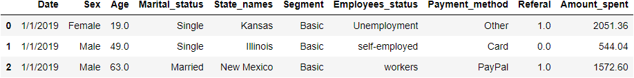
For changing columns name we can use rename() function with passing columns dictionary. In a dictionary, we will pass key like an old column name and value as a new desired column name. For example, now we are going to change Transaction_date and Gender to Date and Sex.

# create new df_col dataframe from df.copy() method. 
df_col = df.copy()

# rename columns name
df_col.rename(columns={"Transaction_date": "Date", "Gender": "Sex"}, inplace=True)
df_col.head(3)

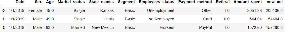
Adding a new column to a Data Frame

You may add a new column to an existing pandas data frame just by assigning values to a new column name. For example, the following code creates a third column named new_col in df_col data frame:

# Add a new_col column which value will be amount_spent * 100
df_col['new_col'] = df_col['Amount_spent'] * 100

df_col.head(3)

String value change or replace

We can replace the new value with the old, with .loc() the method with help of the condition. For Example, now we are changing Female to Woman and Male to Man in Sex column.

df_col.head(3)

# changing Female to Woman and Male to Man in Sex column.
#first argument in loc function is condition and second one is columns name. 
df_col.loc[df_col.Sex == "Female", 'Sex'] = 'Woman' 
df_col.loc[df_col.Sex == "Male", 'Sex'] = 'Man'

df_col.head(3)

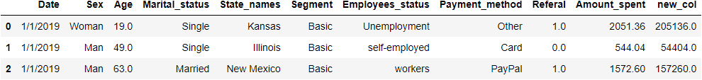
Now Sex columns values are changed Female to Woman and Male to Man.

Datatype change

When we deal with different types of data types sometimes it’s a tedious task. If we want to work on a date we must need to change this with the exact date format. Otherwise, we get the problem. This task is easy on pandas. We can use astype() function to convert one data type to another.

df_col.info()

<class 'pandas.core.frame.DataFrame'>
RangeIndex: 2512 entries, 0 to 2511
Data columns (total 11 columns):
 #   Column            Non-Null Count  Dtype  
---  ------            --------------  -----  
 0   Date              2512 non-null   object 
 1   Sex               2484 non-null   object 
 2   Age               2470 non-null   float64
 3   Marital_status    2512 non-null   object 
 4   State_names       2512 non-null   object 
 5   Segment           2512 non-null   object 
 6   Employees_status  2486 non-null   object 
 7   Payment_method    2512 non-null   object 
 8   Referal           2357 non-null   float64
 9   Amount_spent      2270 non-null   float64
 10  new_col           2270 non-null   float64
dtypes: float64(4), object(7)
memory usage: 216.0+ KB

In our Date columns, it’s object type so now we will convert this to date types, and also we will convert Referal columns float64 to float32.

# change object type to datefime64 format
df_col['Date'] = df_col['Date'].astype('datetime64[ns]')

# change float64 to float32 of Referal columns
df_col['Referal'] = df_col['Referal'].astype('float32')

df_col.info()

<class 'pandas.core.frame.DataFrame'>
RangeIndex: 2512 entries, 0 to 2511
Data columns (total 11 columns):
 #   Column            Non-Null Count  Dtype         
---  ------            --------------  -----         
 0   Date              2512 non-null   datetime64[ns]
 1   Sex               2484 non-null   object        
 2   Age               2470 non-null   float64       
 3   Marital_status    2512 non-null   object        
 4   State_names       2512 non-null   object        
 5   Segment           2512 non-null   object        
 6   Employees_status  2486 non-null   object        
 7   Payment_method    2512 non-null   object        
 8   Referal           2357 non-null   float32       
 9   Amount_spent      2270 non-null   float64       
 10  new_col           2270 non-null   float64       
dtypes: datetime64[ns](1), float32(1), float64(3), object(6)
memory usage: 206.2+ KB

3.3 Remove duplicate

In the data preprocessing part, we need to remove duplicate entries. For different kinds of reasons sometimes our data frames have multiple duplicate entries. Removing duplicate entries can be easily done with help of the pandas function. First, we use duplicated() function for identifying duplicate entries then we use drop_duplicates() for removing them.

# Display duplicated entries 
df.duplicated().sum()

12

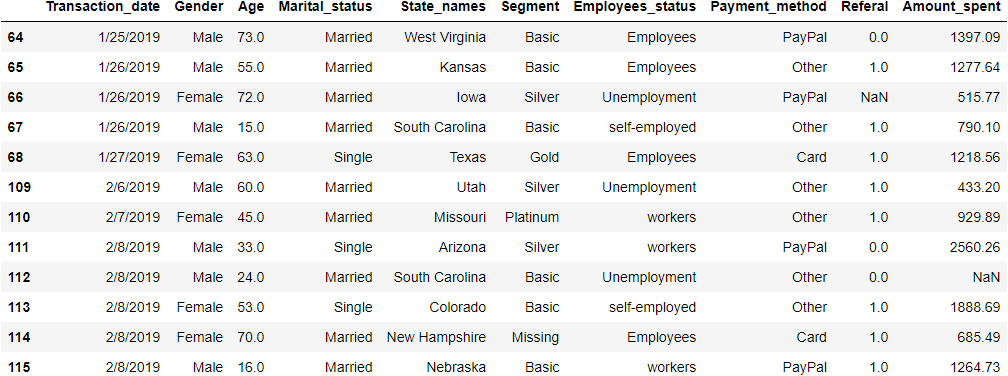
# duplicate rows dispaly, keep arguments will--- 'first', 'last' and False
duplicate_value = df.duplicated(keep='first')

df.loc[duplicate_value, :]

# dropping ALL duplicate values
df.drop_duplicates(keep = 'first', inplace = True)

3.4 Handling missing values

Handling missing values in the common task in the data preprocessing part. For many reasons most of the time we will encounter missing values. Without dealing with this we can’t do the proper model building. For this section first, we will find out missing values then we decided how to handle them. We can handle this by removing affected columns or rows or replacing appropriate values there.

Display missing values information

For displaying missing values we can use isna() function. Counting total missing values in each column in ascending order we use .sum() and sort_values(ascending=False) function.

df.isna().sum().sort_values(ascending=False)

Amount_spent        241
Referal             154
Age                  42
Gender               28
Employees_status     26
Transaction_date      0
Marital_status        0
State_names           0
Segment               0
Payment_method        0
dtype: int64

Delete Nan rows

If we have less Nan value then we can delete entire rows by dropna() function. For this function, we will add columns name in subset parameter.

# df copy to df_copy
df_new = df.copy()

#Delete Nan rows of Job Columns
df_new.dropna(subset = ["Employees_status"], inplace=True)

Delete entire columns

If we have a large number of Nan values in particular columns then dropping those columns might be a good decision rather than imputing.

df_new.drop(columns=['Amount_spent'], inplace=True)

df_new.isna().sum().sort_values(ascending=False)

Referal             153
Age                  42
Gender               27
Transaction_date      0
Marital_status        0
State_names           0
Segment               0
Employees_status      0
Payment_method        0
dtype: int64

Impute missing values

Sometimes if we delete entire columns that will be not the appropriate approach. Delete columns can affect our model building because we will lose our main features. For imputing we have many approaches so here are some of the most popular techniques.

Method 1 — Impute fixed values like 0, ‘Unknown’ or ‘Missing’ etc. We impute Unknown in Gender columns

df['Gender'].fillna('Unknown', inplace=True)

Method 2 — Impute Mean, Median, and Mode

# Impute Mean in Amount_spent columns
mean_amount_spent = df['Amount_spent'].mean()
df['Amount_spent'].fillna(mean_amount_spent, inplace=True)

#Impute Median in Age column
median_age = df['Age'].median()
df['Age'].fillna(median_age, inplace=True)

# Impute Mode in Employees_status column
mode_emp = df['Employees_status'].mode().iloc[0]
df['Employees_status'].fillna(mode_emp, inplace=True)

Method 3 — Imputing forward fill or backfill by ffill and bfill. In ffill missing value impute from the value of the above row and for bfill it’s taken from the below rows value.

df['Referal'].fillna(method='ffill', inplace=True)

df.isna().sum().sum()

0

Now we deal with all missing values with different methods. So now we haven’t any null values.

4. Memory management

When we work on large datasets, There we get one big issue is a memory problem. We need too large resources for dealing with this. But there are some methods in pandas to deal with this. Here are some methods or strategies to deal with this problem with help of pandas.

Change datatype

From changing one datatype to another we can save lots of memory. One popular trick is to change objects to the category it will reduce our data frame memory drastically.

First, we will copy our previous df data frame to df_memory and we will calculate the total memory usage of this data frame using memory_usage(deep=True) method.

df_memory = df.copy()

memory_usage = df_memory.memory_usage(deep=True)
memory_usage_in_mbs = round(np.sum(memory_usage / 1024 ** 2), 3)
print(f" Total memory taking df_memory dataframe is : {memory_usage_in_mbs:.2f} MB ")

Total memory taking df_memory dataframe is : 1.15 MB

Change object to category data types

Our data frame is small in size. Which is 1.15 MB. Now We will convert our object datatype to category.

# Object datatype to category convert
df_memory[df_memory.select_dtypes(['object']).columns] = df_memory.select_dtypes(['object']).apply(lambda x: x.astype('category'))

# convert object to category
df_memory.info(memory_usage="deep")

<class 'pandas.core.frame.DataFrame'>
Int64Index: 2500 entries, 0 to 2511
Data columns (total 10 columns):
 #   Column            Non-Null Count  Dtype   
---  ------            --------------  -----   
 0   Transaction_date  2500 non-null   category
 1   Gender            2500 non-null   category
 2   Age               2500 non-null   float64 
 3   Marital_status    2500 non-null   category
 4   State_names       2500 non-null   category
 5   Segment           2500 non-null   category
 6   Employees_status  2500 non-null   category
 7   Payment_method    2500 non-null   category
 8   Referal           2500 non-null   float64 
 9   Amount_spent      2500 non-null   float64 
dtypes: category(7), float64(3)
memory usage: 189.1 KB

Now its reduce 1.15 megabytes to 216.6 KB. It’s almost reduced 5.5 times.

Change int64 or float64 to int 32, 16, or 8

By default, pandas store numeric values to int64 or float64. Which takes more memory. If we have to store small numbers then we can change to 64 to 32, 16, and so on. For example, our Referral columns have only 0 and 1 values so for that we don’t need to store at float64. so now we change it to float16.

# Change Referal column datatypes
df_memory['Referal'] = df_memory['Referal'].astype('float32')

# convert object to category
df_memory.info(memory_usage="deep")

<class 'pandas.core.frame.DataFrame'>
Int64Index: 2500 entries, 0 to 2511
Data columns (total 10 columns):
 #   Column            Non-Null Count  Dtype   
---  ------            --------------  -----   
 0   Transaction_date  2500 non-null   category
 1   Gender            2500 non-null   category
 2   Age               2500 non-null   float64 
 3   Marital_status    2500 non-null   category
 4   State_names       2500 non-null   category
 5   Segment           2500 non-null   category
 6   Employees_status  2500 non-null   category
 7   Payment_method    2500 non-null   category
 8   Referal           2500 non-null   float32 
 9   Amount_spent      2500 non-null   float64 
dtypes: category(7), float32(1), float64(2)
memory usage: 179.3 KB

After changing only one column’s data types we reduce 216 KB to 179 KB.

Note: Before changing datatype please make sure it’s consequences.

5. Data Analysis

5.1. Calculating Basic statistical measurement

In the data analysis part, we need to calculate some statistical measurements. For calculating this pandas have multiple useful functions. The first useful function is describe() the function it will display most of the basic statistical measurements. For this function, you can add .T for transforming the display. It will make it easy to look at when there are multiple columns.

df.describe().T

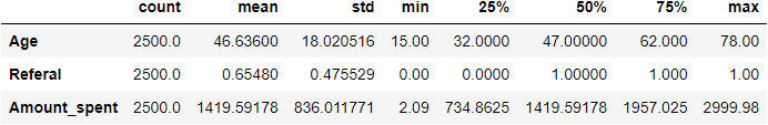
The above function only shows numerical column information. count shows how many values are there. mean shows the average value of each column. std shows the standard deviation of columns, which measures the amount of variation or dispersion of a set of values. min is the minimum value of each column. 25%, 50%, and 75% show total values lie in that groups, and finally max shows maximum values of that columns.

We know already above code will display only numeric columns basic statistical information. for object or category columns we can use describe(include=object) .

df.describe(include=object).T

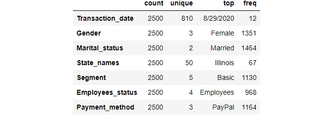
The above information, count shows how many values are there. unique is how many values are unique in that column. The top is the highest number of values lying in that category. freq shows how many values frequently lie on that top values.

We can calculate the mean, median, mode, maximum values, minimum values of individual columns we simply use these functions.

# Calculate Mean
mean = df['Age'].mean()

# Calculate Median
median = df['Age'].median()

#Calculate Mode
mode = df['Age'].mode().iloc[0]

# Calculate standard deviation
std = df['Age'].std()

# Calculate Minimum values
minimum = df['Age'].min()

# Calculate Maximum values
maximum = df.Age.max()

print(f" Mean of Age : {mean}")
print(f" Median of Age : {median}")
print(f" Mode of Age : {mode}")
print(f" Standard deviation of Age : {std:.2f}")
print(f" Maximum of Age : {maximum}")
print(f" Menimum of Age : {minimum}")

Mean of Age : 46.636
 Median of Age : 47.0
 Mode of Age : 47.0
 Standard deviation of Age : 18.02
 Maximum of Age : 78.0
 Menimum of Age : 15.0

In pandas, we can display the correlation of different numeric columns. For this, we can use .corr() function.

# calculate correlation
df.corr()

5.2 Basic built-in function for data analysis

In pandas, there are so many useful basic functions available for data analysis. In this section, we are exploring some of the most frequently used functions.

Number of unique values in the category column

To display the sum of all unique values we use nunique() the function of desired columns name. For example, display total unique values in State_names columns we use this function:

# for display how many unique values are there in State_names column
df['State_names'].nunique()

50

Shows all unique values

To display all unique values we use unique() function with the desired column name.

# for display uniqe values of State_names column
df['State_names'].unique()

array(['Kansas', 'Illinois', 'New Mexico', 'Virginia', 'Connecticut',
       'Hawaii', 'Florida', 'Vermont', 'California', 'Colorado', 'Iowa',
       'South Carolina', 'New York', 'Maine', 'Maryland', 'Missouri',
       'North Dakota', 'Ohio', 'Nebraska', 'Montana', 'Indiana',
       'Wisconsin', 'Alabama', 'Arkansas', 'Pennsylvania',
       'New Hampshire', 'Washington', 'Texas', 'Kentucky',
       'Massachusetts', 'Wyoming', 'Louisiana', 'North Carolina',
       'Rhode Island', 'West Virginia', 'Tennessee', 'Oregon', 'Alaska',
       'Oklahoma', 'Nevada', 'New Jersey', 'Michigan', 'Utah', 'Arizona',
       'South Dakota', 'Georgia', 'Idaho', 'Mississippi', 'Minnesota',
       'Delaware'], dtype=object)

Counts of unique values

To show unique values count we use value_counts() method. This function will display unique values with a number of each value that occurs. For example, if we want to know how many unique values of Gender columns with value frequency number of then we use this method below.

df['Gender'].value_counts()

Female     1351
Male       1121
Unknown      28
Name: Gender, dtype: int64

If we want to show with the percentage of occurrence rather number than we use normalize=True argument in value_counts() function

# Calculate percentage of each category
df['Gender'].value_counts(normalize=True)

Female     0.5404
Male       0.4484
Unknown    0.0112
Name: Gender, dtype: float64

df['State_names'].value_counts().sort_values(ascending = False).head(20)

Illinois         67
Georgia          64
Massachusetts    63
Maine            62
Kentucky         59
Minnesota        59
Delaware         56
Missouri         56
New York         55
New Mexico       55
Arkansas         55
California       55
Arizona          55
Nevada           55
Vermont          54
New Jersey       53
Oregon           53
Florida          53
West Virginia    53
Washington       52
Name: State_names, dtype: int64

Sort values

If we want to sort data frames by particular columns, we need to use sort_values() the method. We can use sort by ascending or descending order. By default, it’s in ascending order. If we want to use descending order then simply we need to pass ascending=False argument in sort_values() the function.

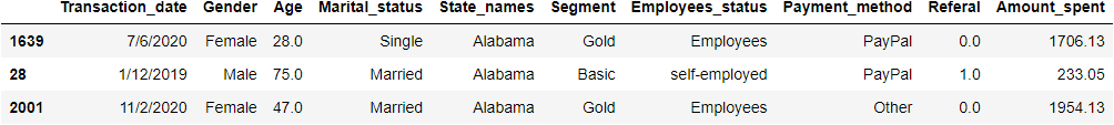
# Sort Values by State_names
df.sort_values(by=['State_names']).head(3)

For sorting our data frame by Amount_spent with ascending order:

# Sort Values Amount_spent with ascending order
df.sort_values(by=['Amount_spent']).head(3)

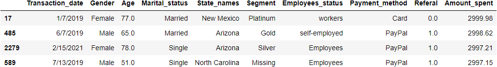
For sorting our data frame by Amount_spent with descending order:

# Sort Values Amount_spent with descending order
df.sort_values(by=['Amount_spent'], ascending=False).head(3)

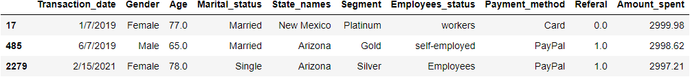
Alternatively, We can use nlargest() and nsmallest() functions for displaying largest and smallest values with desired numbers. for example, If we want to display the 4 largest Amount_spent rows then we use this:

# nlargest
df.nlargest(4, 'Amount_spent').head(10) # first argument is how many rows you want to disply and second one is columns name

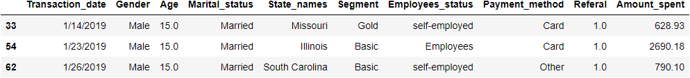
For 3 smallest Amount_spent rows

# nsmallest
df.nsmallest(3, 'Age').head(10)

Conditional queries on Data

If we want to apply a single condition then first we will give one condition then we pass on the data frame. For example, if we want to display all rows where Payment_method is PayPal then we use this:

# filtering - Only show Paypal users
condition = df['Payment_method'] == 'PayPal'
df[condition].head(4)

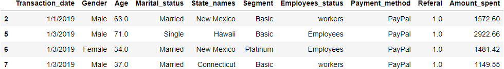
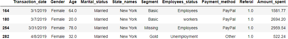
We can apply multiple conditional queries like before. For example, if we want to display all Married female people who lived in New York then we use the following:

# first create 3 condition
female_person = df['Gender'] == 'Female'
married_person = df['Marital_status'] == 'Married'
loc_newyork = df['State_names'] == 'New York'

# we passing condition on our dataframe
df[female_person & married_person & loc_newyork].head(4)

5.3 Summarizing or grouping data

Group by

In Pandas group by function is more popular in data analysis parts. It allows to split and group data, apply a function, and combine the results. We can understand this function and use by below example:

Grouping by one column: For example, if we want to find maximum values of Age and Amount_spent by Gender then we can use this:

df[['Age', 'Amount_spent']].groupby(df['Gender']).max()

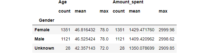
To find mean, count, and max values of Age and Amount_spent by Gender then we can use agg() function with groupby() .

# Group by one columns
state_gender_res = df[['Age','Gender','Amount_spent']].groupby(['Gender']).agg(['count', 'mean', 'max'])
state_gender_res

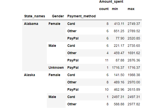
Grouping by multiple columns: To find total count, maximum and minimum values of Amount_spent by State_names, Gender, and Payment_method then we can pass these columns names under groupby() function and add .agg() with count, mean, max argument.

#Group By multiple columns
state_gender_res = df[['State_names','Gender','Payment_method','Amount_spent']].groupby([ 'State_names','Gender', 'Payment_method']).agg(['count', 'min', 'max'])
state_gender_res.head(12)

Cross Tabulation (Cross tab)

Cross tabulation(also referred to as cross tab) is a method to quantitatively analyze the relationship between multiple variables. Also known as contingency tables. It will help to understand the correlation between different variables. For creating this table pandas have a built-in function crosstab().

For creating a simple cross tab between Maritatal_status and Payment_method columns we just use crosstab() with both column names.

pd.crosstab(df.Marital_status, df.Payment_method)

We can include subtotals by margins parameter:

pd.crosstab(df.Marital_status, df.Payment_method, margins=True, margins_name="Total")

If We want a display with percentage than normalize=True parameter help

pd.crosstab(df.Marital_status, df.Payment_method, normalize=True, margins=True, margins_name="Total")

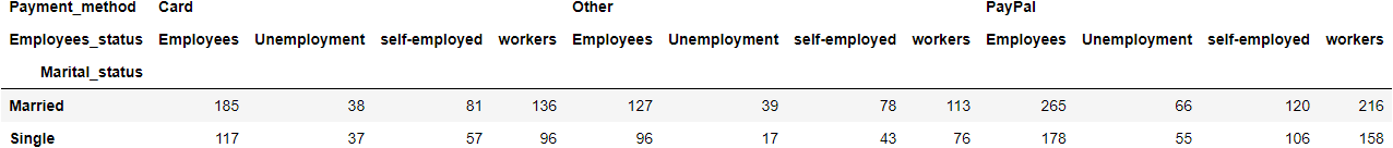
In these cross tab features, we can pass multiple columns names for grouping and analyzing data. For instance, If we want to see how the Payment_method and Employees_status are distributed by Marital_status then we will pass these columns’ names in crosstab() function and it will show below.

pd.crosstab(df.Marital_status, [df.Payment_method, df.Employees_status])

6. Data Visualization

Visualization is the key to data analysis. The most popular python package for visualization is matplotlib and seaborn but sometimes pandas will be handy for you. Pandas also provide some visualization plots easily. For the basic analysis part, it will be easy to use. For this section, we are exploring some different types of plots using pandas. Here are the plots.

6.1 Line plot

A line plot is the simplest of all graphical plots. A line plot is utilized to follow changes over a continuous-time and show information as a series. Line charts are ideal for comparing multiple variables and visualizing trends for single and multiple variables.

For creating a line plot in pandas we use .plot() two columns’ names for the argument. For example, we create a line plot from one dummy dataset.

dict_line = {
    'year': [2016, 2017, 2018, 2019, 2020, 2021],
    'price': [200, 250, 260, 220, 280, 300]
}
df_line = pd.DataFrame(dict_line)

# use plot() method on the dataframe
df_line.plot('year', 'price');

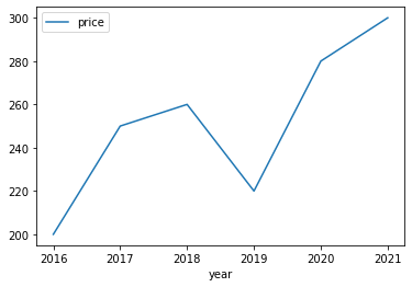
The above line chart shows prices over a different time. It shows like price trend.

6.2 Bar plot

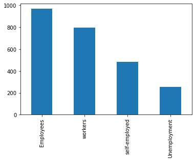
A bar plot is also known as a bar chart shows quantitative or qualitative values for different category items. In a bar, plot data are represented in the form of bars. Bars length or height are used to represent the quantitative value for each item. Bar plot can be plotted horizontally or vertically. For creating these plots look below.

For horizontal bar:

df['Employees_status'].value_counts().plot(kind='bar');

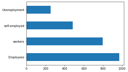
For vertical bar:

df['Employees_status'].value_counts().plot(kind='barh');

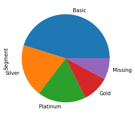
6.3 Pie plot

A pie plot is also known as a pie chart. A pie plot is a circular graph that represents the total value with its components. The area of a circle represents the total value and the different sectors of the circle represent the different parts. In this plot, the data are expressed as percentages. Each component is expressed as a percentage of the total value.

In pandas for creating pie plot. We use kind=pie in plot() function in data frame column or series.

df['Segment'].value_counts().plot(
    kind='pie');

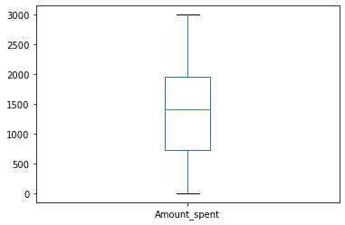
6.4 Box Plot

A box plot is also known as a box and whisker plot. This plot is used to show the distribution of a variable based on its quartiles. Box plot displays the five-number summary of a set of data. The five-number summary is the minimum, first quartile, median, third quartile, and maximum. It will also be popular to identify outliers.

We can plot this by one column or multiple columns. For multiple columns, we need to pass columns name in y variable as a list.

df.plot(y=['Amount_spent'], kind='box');

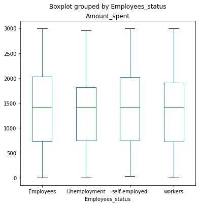
In a box plot, we can plot the distribution of categorical variables against a numerical variable and compare them. Let’s plot it with the Employees_status and Amount_spent columns with pandas boxplot() method:

import matplotlib.pyplot as plt

np.warnings.filterwarnings('ignore', category=np.VisibleDeprecationWarning) 
fig, ax = plt.subplots(figsize=(6,6)) 

df.boxplot(by ='Employees_status', column =['Amount_spent'],ax=ax, grid = False);

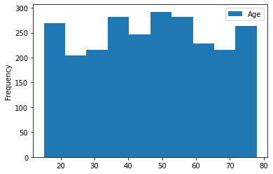
6.5 Histogram

A histogram shows the frequency and distribution of quantitative measurement across grouped values for data items. It is commonly used in statistics to show how many of a certain type of variable occurs within a specific range or bucket. Below we will plot a histogram for looking at Age distribution.

df.plot(
    y='Age',
    kind='hist',
    bins=10
);

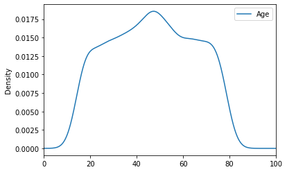
6.6 KDE plot

A kernel density estimate (KDE) plot is a method for visualizing the distribution of observations in a data set, analogous to a histogram. KDE represents the data using a continuous probability density curve in one or more dimensions.

df.plot(
    y='Age',
    xlim=(0, 100),
    kind='kde'
);

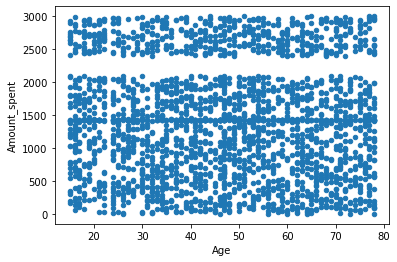
6.7 Scatter plot

A scatter plot is used to observe and show relationships between two quantitative variables for different category items. Each member of the data set gets plotted as a point whose x-y coordinates relate to its values for the two variables. Below we will plot a scatter plot to display relationships between Age and Amount_spent columns.

df.plot(
    x='Age',
    y='Amount_spent',
    kind='scatter'
);

7. Final Thoughts

In this article, we know how pandas can be used to read, preprocess, analyze, and visualize data. It can be also used for memory management for fast computing with fewer resources. The main motive of this article is to help peoples who are curious to learn pandas for data analysis.

Do you have any queries or help related to this article please feel free to contact me on LinkedIn. If you find this article helpful then please follow me for further learning. Your suggestion and feedback are always welcome. Thank you for reading my article. Have wonderful learning.

Feel free to check out GitHub repo for this tutorial.

8. Reference

1. Pandas user guide
2. Pandas 1.x Cookbook
3. The Data Wrangling Workshop
4. Python for Data Analysis
5. Data Analysis with Python: Zero to Pandas — Jovian YouTube Channel
6. Best practices with pandas — Data School YouTube Channel
7. Pandas Tutorials — Corey Schafer YouTube Channel
8. Pandas Crosstab Explained

---

Pandas Complete tutorial for data science in 2022 was originally published in Towards AI on Medium, where people are continuing the conversation by highlighting and responding to this story.

 

Join thousands of data leaders on the AI newsletter. It’s free, we don’t spam, and we never share your email address. Keep up to date with the latest work in AI. From research to projects and ideas. If you are building an AI startup, an AI-related product, or a service, we invite you to consider becoming a sponsor.

Published via Towards AI