Inferential Statistics for Data Science: Explained

Last Updated on January 3, 2021 by Editorial Team

Author(s): Suhas V S

Data Science

A quick dive into the different aspects of inferential statistics using python.

In the earlier part, we have seen how to draw meaningful insights into the characteristics of the sample data (If you have missed it, please find the link at the end of this article). Here, we will be taking forward the understanding we have amassed from the sample study to draw appropriate conclusions on the larger population problem.

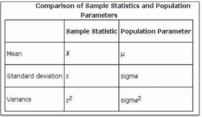
Before moving any further, we need to understand two important terminologies that are parameter and statistic.

Parameter: It is a measure that could be mean, median, variance, and many more for population data.

Statistic: It is a measure that could be mean, median, variance, and many more for sample data.

Relationship between a parameter and a statistic considering the measure “mean”

In real-time, the population data could have millions of observations, which would make the calculations on the entirety of the data complex and slow. Hence, we will be using the statistic measure from the sample data to estimate or test a hypothesis(assumption) about the population parameter.

Example: For example, World Health Organization(WHO) wants to publish a record about the average life longevity of Indians.

So the population contains all the age of all Indians. It is not possible to consider all the Indians( it requires a lot of time and huge amount of money). So we consider a sample of all the Indians.

Now, WHO has decided that the mean age could be an appropriate representation of average life longevity. In this case mean is the parameter. So the Statistics (an appropriate representation of the parameter)will be the mean of the sample.

1.Sampling and its various techniques

Sampling is the process of selecting a sub-group of data points from the population based on a certain logic. This logic is provided by the type of technique used.

Types of Sampling:

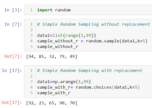
a) Simple Random Sampling: In this type, each of the data points in the population has an equal probability of getting picked up in the sample. It has two methods to do it, namely sampling with replacement(the data point taken in as the first is put back in the sample space before choosing the next data point) and sampling without replacement, which is the converse of the first. Let us see each of them with an example in python.

Note: In sampling with replacement, there are chances of the same data point appearing in the sample which is not the case in sampling without replacement.

Problem: A farmer planted 98 tomato plants last year. He has numbered each plant with numbers 1,2,…98. Now he wants to study the growth of the plants. Help the farmer to select 12 plants randomly as a sample for the study using an appropriate sampling technique. (Refer to figure 2).

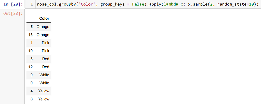
b) Stratified Sampling: Here, the sample data points are selected based on “strata” or commonality. We use “group by” to partition the common data points.

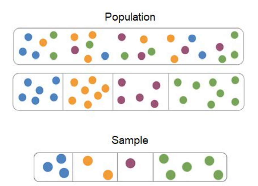
Problem: A rose nursery contains roses of 5 distinct colors. Select two plants of each color randomly.

rose_col = [‘White’, ‘Pink’, ‘White’, ‘Red’, ‘Yellow’, ‘Orange’, ‘Orange’, ‘Red’, ‘Yellow’, ‘White’, ‘Pink’,
‘White’, ‘Red’, ‘Orange’]

c) Systematic Sampling: The first data point is selected randomly and the next one is selected at random intervals.

Problem: Ann has collected 20 beautiful blue marbles pebbles on her last summer vacation. Her mother gave her permission to take only 4 pebbles for her friends. Each of the marble is coded with numbers as 1,2,…20. As 2 is her favorite number, she wants to select pebbles starting from the 2nd pebble. Help Ann to systematically select the 4 marble pebbles for her friends.

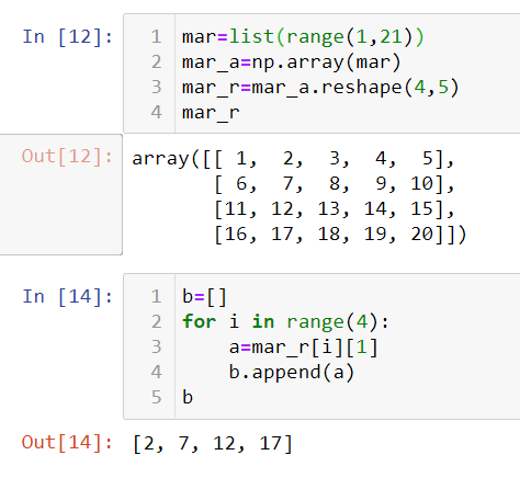
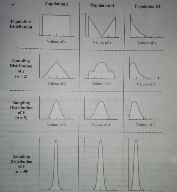
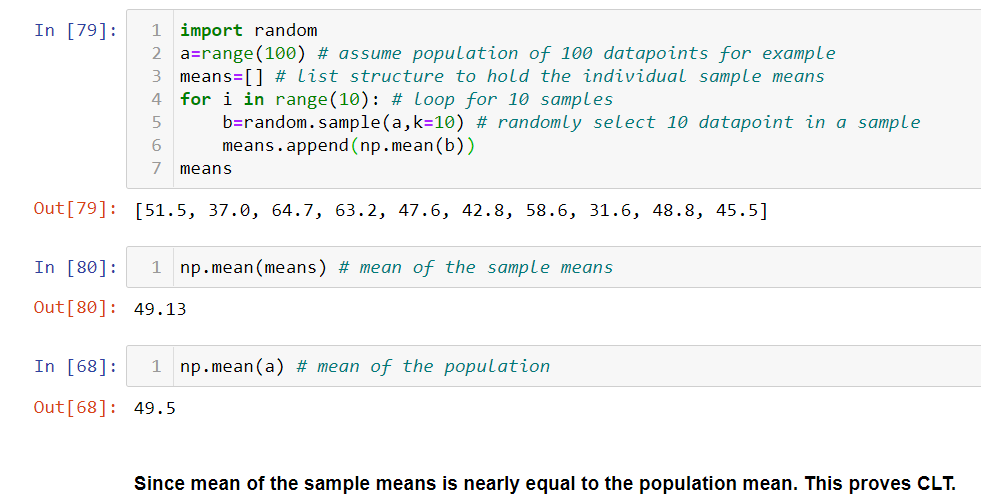
2.Central Limit Theorem

For a large sample size(assume >30), the distribution of the individual means of the samples follows a normal distribution. This is called the “Central Limit Theorem” and the distribution is called “Sampling Distribution”. The means of the samples is called “Sampling Variation”. Also, it states that the mean of the means of the sample is closely near to the mean of the population. These are the important points of the “Central Limit Theorem(CLT)”. The standard deviation of the means of the samples is called “Standard Error”. It is denied by the formula,

Standard Error=σ/√n

where, σ= standard deviation of the population(use sample standard deviation “s” if population standard deviation is unknown), n= sample size

The below figure shows for a sufficiently larger sample size n=30, the sampling distribution follows a “Normal curve”.

Let us prove CLT using a simple example in python,

Requirement:

Total data points=100 , Number of Samples =10, Sample Size =10

3.Estimation

One of the two important parts of inferential statistical analysis is “Estimation” of the population parameter(mean, median, variance, etc). What we generally do is we rigorously work on the sample, calculate the sample statistic and then go on to say that the population parameter could be a certain value(point estimate) or it falls within the range “a” and “b”(interval estimate).

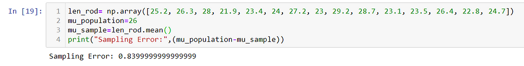
Sampling Error: For a stated value of the population parameter, if we collect some sample data points from the same population and calculate the statistic value for the same measure, the difference between the stated value and the calculated sample value is called “Sampling Error”.

Sampling Error= population parameter-sample statistic

Example: The production manager at the automobile company states that all the steel rods are produced with an average length of 26 cm. Use the data given in the previous question and calculate the sampling error for the mean.

Note: Here , the parameter and statistic measure is “mean”.

Sample,

len_rod (cm) = [25.2, 26.3, 28, 21.9, 23.4, 24, 27.2, 23, 29.2, 28.7, 23.1, 23.5, 26.4, 22.8, 24.7]

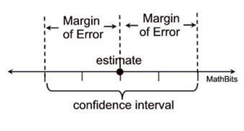
Now, let us come back to the different types of estimates and see their characteristics. The “point estimate” says that the mean of the population is a certain value. This is something we need to look closely at because unless we take the whole population and calculate the “mean”, we would be getting a certain value as the “mean”. Since we are estimating it through a sample of the population, it is bound to have errors in either direction. This is the drawback of “point estimation”.

To overcome this, we say give a range on the negative(Lower limit) and the positive side(Upper limit) of the point estimate according to the error magnitude and say that the population “mean” can lie in between the “lower limit” and the “upper limit”. This is called “interval estimation”.

Let us make it more interesting by assigning a probability value to the interval saying that I am 95% confident that the population mean falls within the range. This interval estimation after assigning a value to it becomes a “Confidence Interval” estimation.

The range of the values from the point estimate on either side till the error magnitude is called “ Margin of Error”. It gives the information as to how far the error is located on either side of the point estimate.

Now that we are comfortable with the above concepts, let us see the mathematical equation for the confidence interval and its components.

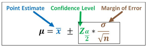
In the above figure, “μ” is the mean of the population in the interval range given by the RHS of the equation. The above equation gives a mathematical assurance to our theory that was explained before that interval estimate is the range of values between the negative(Lower limit) and the positive side(Upper limit) of the point estimate according to the error magnitude.

What is Z_(α/2) in the above equation?

It is the z value providing the area of a/2 of the upper tail of the normal distribution. Also, 1-confidence level=α which is the “level of significance”.

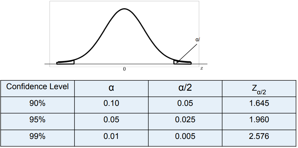
Note: Alternatilvey, you can get the value of Z_(α/2) using python “scipy.stats.norm.isf(α/2)” function. The reason why we take “α/2” instead of “α” is that the normal distribution curve is symmetrical about its mean. The upper and lower tail part can be calculated knowing any one of them. Hence, we take the right part(upper tail) and calculate.

Let us take an example to understand the estimation of the interval using python.

Problem: A pediatrician wants to check the amount of sugar in the 100g pack of baby food produced by KidsGrow company. The medical journal states that a standard deviation of sugar in 100g pack is 8g. The pediatrician collects 37 packets of baby food and found that the average sugar is 24g. Find the 90% confidence interval for the population mean.

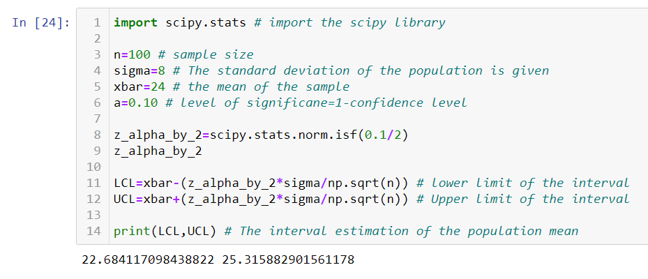
Alternatively, we can use an in-built function to calculate the interval estimate as seen below,

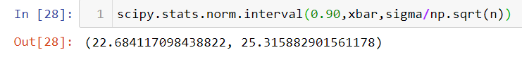
This is all about estimating the interval within which the population “mean” would fall using a “Z-distribution”. This is used when we are aware of the standard deviation of the population(i.e ‘σ’) and the sample size n >30. In case if the “σ” is unknown and the sample size n < 30, then we use a distribution called “T-distribution”.

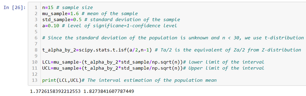
Note: T-distribution is always dependent on what is called a “degree of freedom” of the sample size. If “n” is the sample size, then the degree of freedom is n-1.

Problem: The health magazine in Los Angeles states that a person should drink 1.8 L of water every day. To study this statement, the physician collects the data of 15 people and found that the average water intake for these people is 1.6 L with a standard deviation of 0.5 L. Calculate the 90% confidence interval for the population's average water intake.

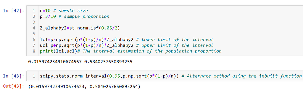
All this while we saw the interval estimation for a numerical variable, now let us see the interval estimation for the categorical variable(i.e for proportion). The assumption we make is that the distribution always follows a normal curve and we use “Z-distribution”.

Problem on proportion: The NY university has opened the post of Astrophysics professor. The total number of applications was 36. To check the authenticity of the applicants a sample of 10 applications was collected, out of which 3 applicants were found to be a fraud. Construct the 95% confidence interval for the population proportion.

4.Hypothesis and HypothesisTesting

What is a Hypothesis?

Hypothesis in statistics is any testable claim or assumption about the parameter of the population. It should be capable of being tested, either by experiment or observation. Example- The new engine developed by R & D gives more mileage than the existing engine.

Type of Hypothesis:

a) Null Hypothesis(H0): In the type, we say that there is no variation in the outcome. That means, there is no real effect.

Examples :

• Special training on students does not affect.
• Different teaching method does not affect students’ performance
• The drug used for headaches does not affect the application.

b) Alternate Hypothesis(Ha): It is the contrasting statement to H0 where it says there is a real effect in the outcome. This is the statement we are trying to prove.

Examples:

• Special training on students has a significant effect.
• Different teaching method has a significant effect on students’ performance.
• The drug used for headaches has a significant effect after application.

Hypothesis Testing Process:

As we already know, a hypothesis is a testable claim and only either H0 or Ha can be proved. The process of proving either of them is called the “Hypothesis Testing Process”. Note that if we accept H0, automatically Ha is rejected and vice-versa.

We assign a confidence level to hypothesis testing and try to limit the amount of error being committed. The universally accepted confidence level is 95%. By doing so we admit that while rejecting the null hypothesis, there is a 5% possibility of wrongly rejecting the null hypothesis.

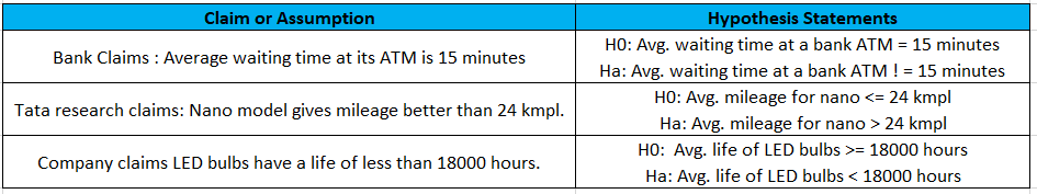
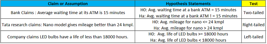
Note: While framing the Hypothesis statements, the equality sign =, ≤, ≥ should always appear on the Null Hypothesis side. With this idea in mind let us write hypothesis statements for a few examples in figure 16.

Hypothesis Testing:

After framing the hypothesis statements H0 and Ha for a given claim, it is now time to prove either of them wrong. This is done by 3 well-defined methods namely,

a) Critical value approach

b) p-value approach

c) Confidence interval approach

Before going further into each of them, we need to understand something called a “left/right-tailed test” or a “two-tailed test”. The trick here is to observe the H0 and Ha statements.

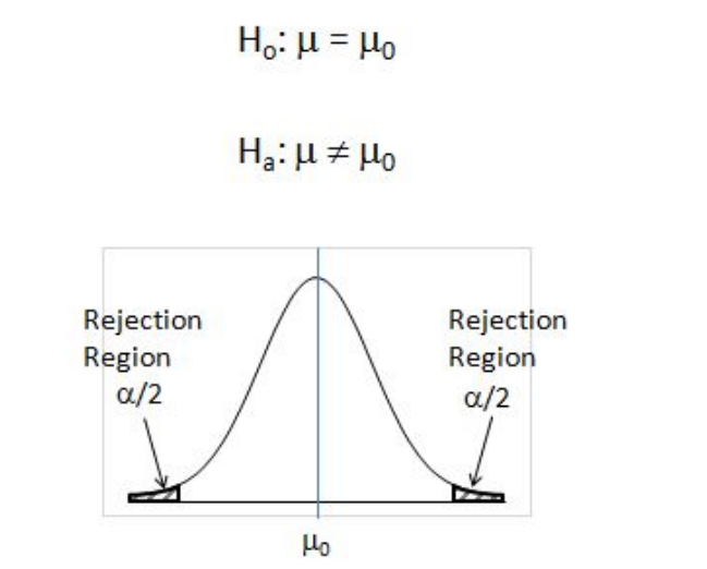
If H0 has an “=” sign in it, it means to say that is a “two-tailed” test. Two-tailed tests are used, when it is required to test if the observed mean is equal to the hypothesized mean.

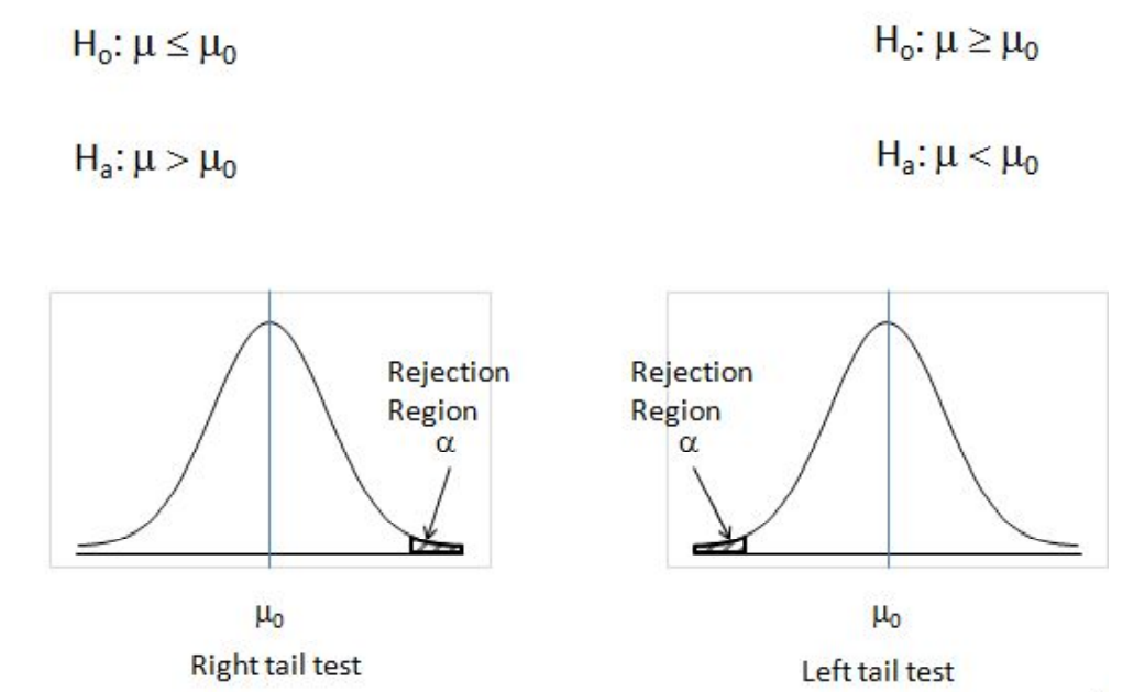
One-tailed tests are used, when it is required to test if the observed mean significantly exceeds the hypothesized mean or when it is significantly lesser than the hypothesized mean. If Ha has a “<” or a “>” sign in it then it is a “left-tailed” and a “right-tailed test” respectively.

a) Critical value approach:

Steps involved:

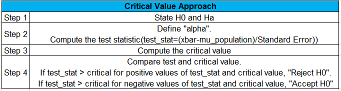
To compute critical values, the kind of test that we observe from the problem statement is very important.

For a left tailed test, the “test_stat” and the “critical” values will lie on the left of the mean of the normal curve. Hence, their values will be negative. Then,

critical= scipy.stats.norm.ppf(α) using Z-distribution for “σ “(known)

critical= scipy.stats.t.ppf(α,n-1) using T-distribution for “σ “(unknown)

For a right-tailed test, the “test_stat” and the “critical” values will lie on the right of the mean of the normal curve. Hence, their values will be positive. Then,

critical= scipy.stats.norm.isf(α) using Z-distribution for “σ “(known)

critical= scipy.stats.t.isf(α,n-1) using T-distribution for “σ “(unknown)

For a two-tailed test, the “test_stat” and the “critical” values can lie on either side of the normal curve. If the test_stat is “negative”, use the formula to calculate the critical value from the left tailed test. The same can be done if the test_stat is “positive”(i.e use the formula to calculate the critical value from the right-tailed test).

To perform step 4, we need to understand the rejection region of H0 for the different tailed test. Refer to figure 20 and 21.

b) p-value approach:

Steps involved:

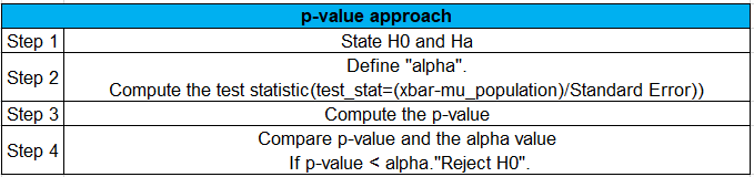
To compute a p-value, the kind of test that we observe from the problem statement is very important.

For a left tailed test, the “test_stat” and the “critical” values will lie on the left of the mean of the normal curve. Hence, their values will be negative. Then,

p_value= scipy.stats.norm.cdf(test_stat) using Z-distribution for “σ “(known)

p_value= scipy.stats.t.cdf(test_stat,n-1) using T-distribution for “σ “(unknown)

For a right-tailed test, the “test_stat” and the “critical” values will lie on the right of the mean of the normal curve. Hence, their values will be positive. Then,

p_value= scipy.stats.norm.sf(test_stat) using Z-distribution for “σ “(known)

p_value= scipy.stats.t.sf(test_stat,n-1) using T-distribution for “σ “(unknown)

For a two-tailed test, the “test_stat” and the “critical” values can lie on either side of the normal curve. If the test_stat is “negative”, use the formula to calculate the p-value from the left tailed test. The same can be done if the test_stat is “positive”(i.e use the formula to calculate the p-value from the right-tailed test). Note that you will have to multiply the p-value by 2 so that it is applicable for both the tails.

c) Confidence Interval approach:

Steps involved:

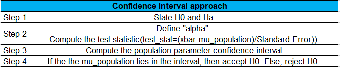
Note: The computation of parameter confidence interval is the same as we had worked in the parameter estimation.

This is all about different types of hypothesis testing. Now, we will take an example work out all the 3 approaches.

Problem: The production manager at tea emporium claims that the weight of a green tea bag is less than 3.5 g. To test the manager’s claim consider a sample of 50 tea bags. The sample average weight is found to be 3.28 g with a standard deviation of 0.6 g. Use the p-value technique to test the claim at a 10% level of significance.

What can we decide on the hypothesis as to which one is correct?

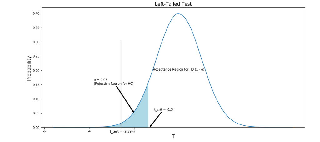
Looking at the plot, we can decide on whether to accept or reject H0. Here is our conclusion comment.

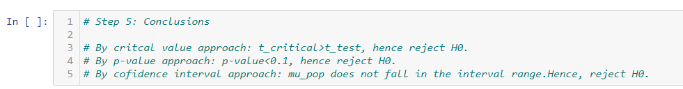
This concludes the parameter estimation and hypothesis testing part of the inferential statistical analysis. These concepts are the fundamentals while working work on advanced statistical techniques involving 2 or more samples for the test of mean and proportion. I hope this will help to lay a basic foundation with inferential statistics. I will continue to write and bring out more interesting topics in the coming future. Till then, happy reading!!!.

If you have missed the first part of the descriptive statistical analysis or would like to give it another read, please find it in the below link.

Descriptive Statistics for Data Science: Explained

---

Inferential Statistics for Data Science: Explained was originally published in Towards AI on Medium, where people are continuing the conversation by highlighting and responding to this story.

Published via Towards AI