Explainable AI: GradCAM

Author(s): Shubham Bhandari

Originally published on Towards AI.

With the recent advancements in AI, we are witnessing the emergence of some of the most sophisticated AI systems that have ever existed. Propelled by the wave of LLMs like ChatGPT, Microsoft Copilot and Google Gemini, these intelligent systems are rapidly evolving. But like everything, even AI comes with some flaws, notably being a black box in some cases.

A black box model is one where the user has no clue about the features the model has considered for making a prediction. The inputs and outputs are known, but the internal workings are unknown. Some examles include deep neural networks like CNN, RNN, LSTM etc.

This article aims at explaining explainable AI (mouthful, huh?) and a solution to explain predictions made by Convolutional Neural Networks. It will demonstrate an implementation of GradCAM using PyTorch and go over the nitty-gritty of this technique.

Sounds interesting? Let’s dive in.

Explainable AI

Let’s start with the basics. What the heck is Explainable AI?

We have been training and using deep neural networks for quite some time now. With their mass adoption, there is a need to make sure that the reason for the model’s prediction is correct. Especially in high-stake cases such as healthcare, finance, and law, where the basis of an AI’s decision is as crucial as the decision itself. In such situations, it is critical to know the reasoning behind the decisions.

The idea behind Explainable AI is to explain the prediction in a way that humans can understand and comprehend. It aims to provide an insight into the “internal” workings of the model. This is to make sure that the results obtained from the model are based on genuine features and not on some peculiar attributes in the training data.

GradCAM

GradCAM (Gradient-weighted Class Activation Mapping) is a popular technique that allows us to visualize the decisions made by Convolutional Neural Networks. The salient features that make it apt for explaining CNN models are as follows:

1. GradCAM shows visual explanations to help us localize a category in the image.
2. It is applicable to various tasks that involve CNN models. Be it image classification, captioning, etc. To top it off, one doesn’t need to retrain or make any architectural changes in the model to use GradCAM.
3. GradCAM helps in distinguishing between stronger and weaker models by showing the features that the respective model considered while making the decision.

Sounds good, but how does it even work?

GradCAM uses the gradients from the final convolutional layer to produce a localization map, highlighting the important regions in the image used for making predictions.

Ahhh… wait what?

Let me elaborate.

1. The first step is Forward Pass: The image gets passed through a CNN to perform computations and generate a score for the desired category.
2. Compute gradients: All the gradients except the category we are interested in are set to 0. For the desired category, the gradient is set to 1. Then, backpropagation is performed through the Rectified Convolutional feature maps of interest.
3. Combine Backward Gradients: The backward gradients are then pooled across both dimensions to calculate the importance of each feature map. These captured weights indicate the importance of each feature map for the target class.
4. Generate Heatmap: This weighted combination is then used to develop a heatmap (localization map). This shows us where the model is looking while making a decision for the desired class.
5. Apply the classic ReLU: A Rectified Linear Unit is then applied to the heatmap to only account for features that have a positive influence on the desired class. This is to ensure that features important to the target class are highlighted. Thus, improving the localization of the “Class Discriminative Regions”.
6. Finally, normalize the heatmap: The result generated from the above steps is then normalized and displayed as an overlay on the test image.

Implementation:

Enough chit-chat; time to get our hands dirty. Let’s combine all the above steps to create our own GradCAM implementation using PyTorch.

Sweet! But the question arises how will we get gradients?

Here comes Hooks for the rescue.

PyTorch Hooks

Hooks are powerful tools for monitoring the neural network during forward as well as backward propagation. They can be used for extracting intermediate data and debugging. There are two types of hooks available:

1. Forward Hooks: Executed during a forward pass. Capable of extracting or modifying the output of layers.
2. Backward Hooks: Executed during back-propagation. Useful in inspecting and modifying the gradients obtained during back-propagation.

In action:

The next step is to tie the hooks and GradCAM together:

The example demonstrated uses the ResNet-152 architecture. It is a variant of Residual Network architecture (a type of CNN) comprising 152 layers designed for tasks in the field of computer vision. We will use the pre-trained model provided by PyTorch and perform object detection. Ideally, the model will detect the object, and GradCAM will produce a heatmap overlaying the original image.

The final layer in the case of ResNet is layer 4. The hooks are registered to this layer for obtaining weights and gradients. Here is a snippet of the structure of the model:

(layer4): Sequential(
 (0): Bottleneck(
 (conv1): Conv2d(1024, 512, kernel_size=(1, 1), stride=(1, 1), bias=False)
 (bn1): BatchNorm2d(512, eps=1e-05, momentum=0.1, affine=True, track_running_stats=True)
 (conv2): Conv2d(512, 512, kernel_size=(3, 3), stride=(2, 2), padding=(1, 1), bias=False)
 (bn2): BatchNorm2d(512, eps=1e-05, momentum=0.1, affine=True, track_running_stats=True)
 (conv3): Conv2d(512, 2048, kernel_size=(1, 1), stride=(1, 1), bias=False)
 (bn3): BatchNorm2d(2048, eps=1e-05, momentum=0.1, affine=True, track_running_stats=True)
 (relu): ReLU(inplace=True)
 (downsample): Sequential(
 (0): Conv2d(1024, 2048, kernel_size=(1, 1), stride=(2, 2), bias=False)
 (1): BatchNorm2d(2048, eps=1e-05, momentum=0.1, affine=True, track_running_stats=True)
 )
 )
 (1): Bottleneck(
 (conv1): Conv2d(2048, 512, kernel_size=(1, 1), stride=(1, 1), bias=False)
 (bn1): BatchNorm2d(512, eps=1e-05, momentum=0.1, affine=True, track_running_stats=True)
 (conv2): Conv2d(512, 512, kernel_size=(3, 3), stride=(1, 1), padding=(1, 1), bias=False)
 (bn2): BatchNorm2d(512, eps=1e-05, momentum=0.1, affine=True, track_running_stats=True)
 (conv3): Conv2d(512, 2048, kernel_size=(1, 1), stride=(1, 1), bias=False)
 (bn3): BatchNorm2d(2048, eps=1e-05, momentum=0.1, affine=True, track_running_stats=True)
 (relu): ReLU(inplace=True)
 )
 (2): Bottleneck(
 (conv1): Conv2d(2048, 512, kernel_size=(1, 1), stride=(1, 1), bias=False)
 (bn1): BatchNorm2d(512, eps=1e-05, momentum=0.1, affine=True, track_running_stats=True)
 (conv2): Conv2d(512, 512, kernel_size=(3, 3), stride=(1, 1), padding=(1, 1), bias=False)
 (bn2): BatchNorm2d(512, eps=1e-05, momentum=0.1, affine=True, track_running_stats=True)
 (conv3): Conv2d(512, 2048, kernel_size=(1, 1), stride=(1, 1), bias=False)
 (bn3): BatchNorm2d(2048, eps=1e-05, momentum=0.1, affine=True, track_running_stats=True)
 (relu): ReLU(inplace=True)
 )
 )

Aaannddd… that’s about it, let’s see GradCAM in action:

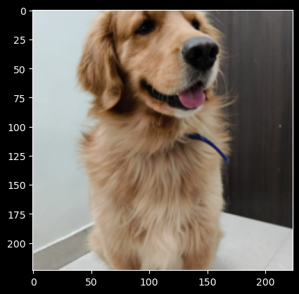
Our first test image is this Golden Retriever Coco. Isn’t he the most handsome? U+1F60D:

Prediction: 207, 'golden retriever', 8.249414

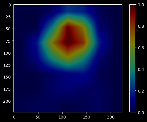
Values closer to 1 signify a feature being used for prediction, and features for which values are closer to 0 are not being used by the model. The result is close to what a human brain will consider to identify the breed of the dog. So far, so good.

Then, we have this super cute Siberian Husky pup:

Prediction: 250, 'Siberian husky', 8.082574

It looks good, and the highlighted features are as expected.

Moving on, let us see an interesting example: The original image shows a tiger cat lying on a doormat. The model correctly identifies both values: doormat and tiger cat. For the doormat, it considers features around the cat as shown in the image. For the tiger-cat prediction, the model focuses on the cat.

This demonstrates the capability of GradCAM and how it can be used to show the basis of prediction by a CNN model.

Credits to my friends for providing their furry friend’s photos.

Head over to the repository to test and check out the complete implementation of GradCAM with its usage.

That’s a wrap! Thanks for reading. Your reviews are always welcome. Cheers!

References:

https://arxiv.org/pdf/1610.02391.pdf

https://pytorch.org/tutorials/beginner/former_torchies/nnft_tutorial.html

Join thousands of data leaders on the AI newsletter. Join over 80,000 subscribers and keep up to date with the latest developments in AI. From research to projects and ideas. If you are building an AI startup, an AI-related product, or a service, we invite you to consider becoming a sponsor.

Published via Towards AI