


Exploratory Data Analysis: Baby Steps
Last Updated on November 18, 2020 by Editorial Team
Author(s): Swetha Lakshmanan

Data science is often thought to consist of advanced statistical and machine learning techniques. However, another key component to any data science endeavor is often undervalued or forgotten: exploratory data analysis (EDA). It is a classical and under-utilized approach that helps you quickly build a relationship with the new data.
It is always better to explore each data set using multiple exploratory techniques and compare the results. This step aims to understand the dataset, identify the missing values & outliers if any using visual and quantitative methods to get a sense of the story it tells. It suggests the next logical steps, questions, or areas of research for your project.
Steps in Data Exploration and Preprocessing:
- Identification of variables and data types
- Analyzing the basic metrics
- Non-Graphical Univariate Analysis
- Graphical Univariate Analysis
- Bivariate Analysis
- Variable transformations
- Missing value treatment
- Outlier treatment
- Correlation Analysis
- Dimensionality Reduction
I will discuss the first 4 steps in this article and the rest in the upcoming articles.
Dataset:
To share my understandings and techniques, I know, I’ll take an example of a dataset from a recent Analytics Vidhya Website’s competition — Loan Default Challenge. Let’s try to catch hold of a few insights from the data set using EDA.
I have used a subset of the original dataset for this analysis. You can download it here.
The original dataset can be found here.
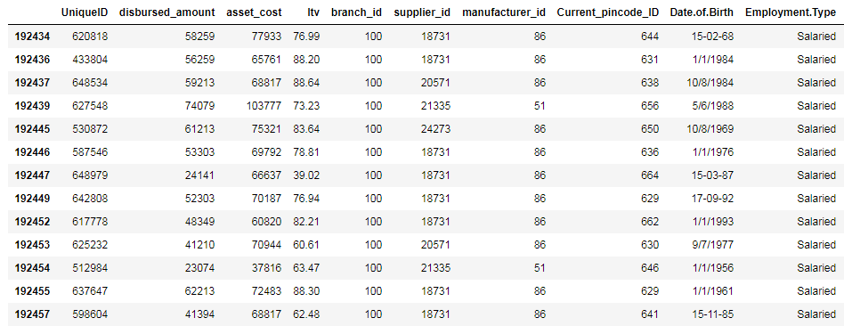
The sample dataset contains 29 columns and 233155 rows.
Variable identification:
The very first step in exploratory data analysis is to identify the type of variables in the dataset. Variables are of two types — Numerical and Categorical. They can be further classified as follows:

Once the type of variables is identified, the next step is to identify the Predictor (Inputs) and Target (output) variables.
In the above dataset, the numerical variables are,
Unique ID, disbursed_amount, asset_cost, ltv, Current_pincode_ID, PERFORM_CNS.SCORE, PERFORM_CNS.SCORE.DESCRIPTION, PRI.NO.OF.ACCTS, PRI.ACTIVE.ACCTS, PRI.OVERDUE.ACCTS, PRI.CURRENT.BALANCE, PRI.SANCTIONED.AMOUNT, PRI.DISBURSED.AMOUNT, NO.OF_INQUIRIES
And the categorical variables are,
branch_id, supplier_id, manufacturer_id, Date.of.Birth, Employment.Type, DisbursalDate, State_ID, Employee_code_ID, MobileNo_Avl_Flag, Aadhar_flag, PAN_flag, VoterID_flag, Driving_flag, Passport_flag, loan_default
The target value is loan_default, and the rest 28 features can be assumed as the predictor variables.
The data dictionary with the description of all the variables in the dataset can be found here.
Importing Libraries:
#importing libraries
import pandas as pd
import numpy as np
import matplotlib as plt
import seaborn as sns
Pandas library is a data analysis tool used for data manipulation, Numpy for scientific computing, and Matplotlib & Seaborn for data visualization.
Importing Dataset:
train = pd.read_csv("train.csv")
Let’s import the dataset using the read_csv method and assign it to the variable ‘train.’
Identification of data types:
The .dtypes method to identify the data type of the variables in the dataset.
train.dtypes
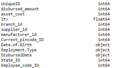
Both Date.of.Birth and DisbursalDate are of the object type. We have to convert it to DateTime type during data cleaning.
Size of the dataset:
We can get the size of the dataset using the .shape method.
train.shape
Statistical Summary of Numeric Variables:
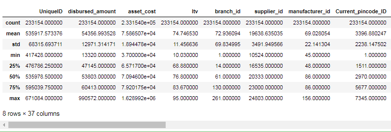
Pandas describe() is used to view some basic statistical details like count, percentiles, mean, std, and maximum value of a data frame or a series of numeric values. As it gives the count of each variable, we can identify the missing values using this method.
train.describe()
Non-Graphical Univariate Analysis:
To get the count of unique values:
The value_counts() method in Pandas returns a series containing the counts of all the unique values in a column. The output will be in descending order so that the first element is the most frequently-occurring element.
Let’s apply value counts to the loan_default column.
train['loan_default'].value_counts()


To get the list & number of unique values:
The nunique() function in Pandas returns a series with several distinct observations in a column.
train['branch_id'].nunique()
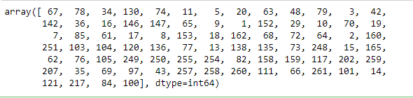
Similarly, the unique() function of pandas returns the list of unique values in the dataset.
train['branch_id'].unique()
Filtering based on Conditions:
Datasets can be filtered using different conditions, which can be implemented using logical operators in python. For example, == (double equal to), ≤ (less than or equal to), ≥(greater than or equal to), etc.
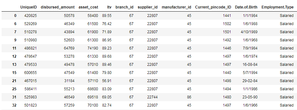
Let’s apply the same to our dataset and filter out the column which has the Employment.Type as “Salaried”
train[(train['Employment.Type'] == "Salaried")]
Now let’s filter out the records based on two conditions using the AND (&) operator.
train[(train['Employment.Type'] == "Salaried") & (train['branch_id'] == 100)]
You can try out the same example using the OR operator (|) as well.
Finding null values:
When we import our dataset from a CSV file, many blank columns are imported as null values into the Data Frame, which can later create problems while operating that data frame. Pandas isnull() method is used to check and manage NULL values in a data frame.
train.apply(lambda x: sum(x.isnull()),axis=0)
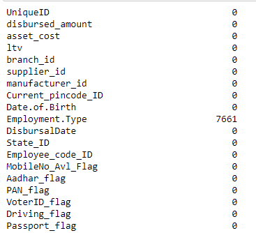
We can see that there are 7661 missing records in the column ‘Employment.Type’. These missing records should be either deleted or imputed in the data preprocessing stage. I will talk about different ways to handle missing values in detail in my next article.
Data Type Conversion using to_datetime() and astype() methods:
Pandas astype() method is used to change the data type of a column. to_datetime() method is used to change, particularly to DateTime type. When the data frame is imported from a CSV file, the data type of the columns is set automatically, which many times is not what it actually should have. For example, in the above dataset, Date.of.Birth and DisbursalDate are both set as object type, but they should be DateTime.
Example of to_datetime():
train['Date.of.Birth']= pd.to_datetime(train['Date.of.Birth'])
Example of astype():
train['ltv'] = train['ltv'].astype('int64')
Graphical Univariate Analysis:
Histogram:
Histograms are one of the most common graphs used to display numeric data. Histograms two important things we can learn from a histogram:
- distribution of the data — Whether the data is normally distributed or if it’s skewed (to the left or right)
- To identify outliers — Extremely low or high values that do not fall near any other data points.
Lets plot histogram for the ‘ltv’ feature in our dataset
train['ltv'].hist(bins=25)

Here, the distribution is skewed to the left.
train['asset_cost'].hist(bins=200)
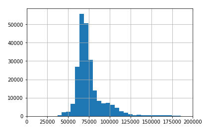
The above one is a normal distribution with a few outliers in the right end.
Box Plots:
A Box Plot is the visual representation of the statistical summary of a given data set.
The Summary includes:
- Minimum
- First Quartile
- Median (Second Quartile)
- Third Quartile
- Maximum
It is also used to identify the outliers in the dataset.

Example:
print(train.boxplot(column='disbursed_amount'))
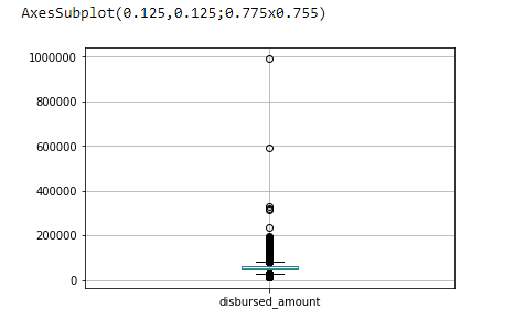
Here we can see that the mean is around 50000. There are also few outliers at 60000 and 1000000, which should be treated in the preprocessing stage.
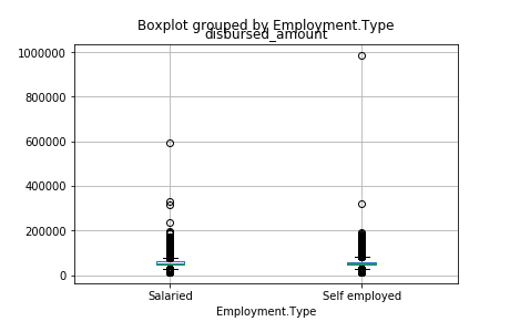
train.boxplot(column=’disbursed_amount’, by = ‘Employment.Type’)
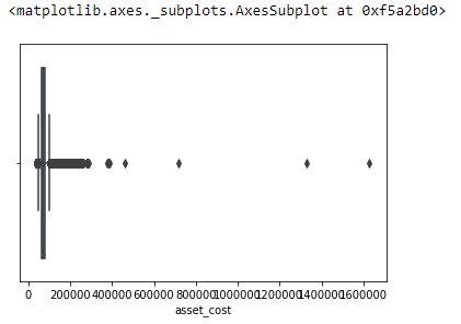
sns.boxplot(x=train['asset_cost'])
Count Plots:
A count plot can be thought of as a histogram across a categorical, instead of numeric, variable. It is used to find the frequency of each category.
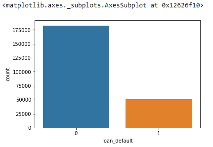
sns.countplot(train.loan_default)
sns.countplot(train.manufacturer_id)
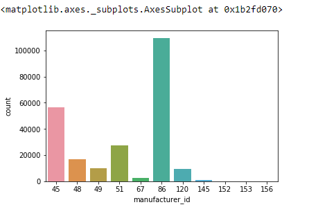
Here we can see that category “86” is dominating over the other categories.
These are the basic, initial steps in exploratory data analysis. I wish to cover the rest of the steps in the next few articles. I hope you found this short article helpful.
Towards AI Academy
We Build Enterprise-Grade AI. We'll Teach You to Master It Too.
15 engineers. 100,000+ students. Towards AI Academy teaches what actually survives production.
Start free — no commitment:
→ 6-Day Agentic AI Engineering Email Guide — one practical lesson per day
→ Agents Architecture Cheatsheet — 3 years of architecture decisions in 6 pages
Our courses:
→ AI Engineering Certification — 90+ lessons from project selection to deployed product. The most comprehensive practical LLM course out there.
→ Agent Engineering Course — Hands on with production agent architectures, memory, routing, and eval frameworks — built from real enterprise engagements.
→ AI for Work — Understand, evaluate, and apply AI for complex work tasks.
Note: Article content contains the views of the contributing authors and not Towards AI.
Related posts

")


Recent Posts


")


Comments are closed.