Breaking Down Mistral 7B ⚡🍨

Author(s): JAIGANESAN

Originally published on Towards AI.

Breaking Down Mistral 7B ⚡🍨

In this article, we’ll delve into the Mistral architecture, exploring its unique features and how it differs from other open-source large language models (LLMs).

If you are wondering where this architecture comes from, I recommend you to check out the Mistral inference Github code and Research paper.

GitHub – mistralai/mistral-inference: Official inference library for Mistral models

Official inference library for Mistral models. Contribute to mistralai/mistral-inference development by creating an…

github.com

Before we begin, it’s essential to have a basic understanding of how LLMs work and their functionality. If you’re new to this topic, I recommend checking out my previous article, Large Language Models: In and Out, which covers the basics of LLM functioning, Embedding, self-attention, multi-head attention, and RMS Normalization. I won’t be covering these topics in this article, so please take a moment to familiarize yourself with the basics. 😊

Large Language Model (LLM)🤖: In and Out

Delving into the Architecture of LLM: Unraveling the Mechanics Behind Large Language Models like GPT, LLAMA, etc.

pub.towardsai.net

Let’s take a closer look at the Mistral architecture. This architecture has a model dimension of 4096. It’s made up of 32 layers. The model uses 32 heads and 8 key value (KV) heads. Each head in the model has a dimension of 128. The feed-forward network (FFN) has a hidden dimension of 14336. The sliding window size is set to 4096. The context length is 8192 and the vocabulary size is 32000 😯.

In this article, we’ll focus on the following concepts that make Mistral architecture stand out:

✨ Rotary Positional Encoding

✨ Sliding Window Attention

✨ Grouped Query Attention

✨ Feed Forward Network in Mistral 7B

✨ SiLU Activation Function.

✨ KV Cache and KV Cache with Rolling Buffer cache

✨ Linear Layer and softmax activation

Let’s dive deeper into each of these concepts and explore what makes Mistral architecture so unique and attractive to the AI community.

1. Rotary Positional Encoding (RoPE) 🦸‍♂

First, why do we need Positional Encoding? Without positional Encoding, the transformer model cannot differentiate between the same word in different positions. 🤷‍♂

Before we dive into rotary positional encoding, let’s first understand relative positional encoding. We have seen sinusoidal functions in the traditional Transformer model [2] to calculate positional encoding. However, this approach has a limitation — it’s more absolute, less relative, and doesn’t change for every batch. It represents only its position.

Same Positional Embedding vector for all batches. Each token in the sequence has its positional embedding, which doesn’t consider the relationships with other tokens.

On the other hand, relative positional encoding [1] represents the distance between two tokens in a sequence. This helps the attention mechanism understand the relative positions of tokens, rather than just their absolute positions. It focuses on two tokens at a time and is involved in the attention calculation process. The attention mechanism captures how one word relates to another using attention scores, which rely on the relative distances between tokens.

x in image 2, is the input sequence vector. i and j represent individual vectors. a_ij_K represents the distance between two vectors or tokens. e_ij is the attention score. Formula in Image 2, Implementation of relative position in multi-head attention.

Let’s consider a simple example to illustrate this concept. Imagine 100 people standing in a straight line. I’m standing in the 10th position, my friend is standing in the 40th position, and another friend is standing in the 74th position. In the traditional Transformer model, we would feed the position of each input token as 1, 2,…, 10,…, 40,…, 74,…, 100. It’s all independent from each other.

However, relative positional encoding takes a different approach. Instead of focusing on the absolute positions, it calculates the distance between my friends and me. In this case, the distance between me and my friend in the 40th position is 30 (40–10), and the distance between me and my friend in the 74th position is 64 (74–10) interchangeably my friends to me is (-30,-64). Same as thinking of it in a Multi-dimensional space.

From Images 3 and 4, you can understand how relative positional embedding is implemented between 2 tokens.

Note: * Numbers in the images are illustration purpose only.

First I want to talk about Image 3, i and j represent the two tokens in Query and Key. Let’s think of a dimensions (1,1024). R_(j-i) distance between vectors in the multi-dimensional space. In Multi-head attention, we multiply with weight matrices W_Q, W_K, and W_V to create head vectors as shown in image 2. A point to note is that Relative positional embedding could be learnable. There is a Clip method applied to calculate distance if the distance is too large between vectors.

Then why, do we need Rotary Positional encoding? Because Relative positional encoding is computationally inefficient 😔(We need to give an extra positional encoding matrix in the Attention mechanism) and It is not suitable for inference (Nowadays LLMs use the KV cache method) so the relative position is not the best solution.

There comes rotary positional embedding. This method combines the best of both worlds — absolute and relative positional embedding. It uses a rotation matrix (r) to rotate the input embeddings, that will be used in the attention mechanism as query and key, not value. This Inner product gives both positional information and attention(Semantic, syntactic) information between vectors.

So, what’s the big deal about this inner product? Well, it only depends on the two vectors and the distance between the tokens they represent. To make this work, we need to find a way to incorporate relative position information. We can do this by using a function g(Rotation), and the word embeddings are x_m and x_n, and their relative position (m-n). This function g will give us the inner product (attention) we need.

But how does this rotation matrix work its magic? Simply put, it rotates a vector to another vector by a certain angle (theta). This is based on the trigonometric properties of sine and cosine. If you take a look at Images 6 and 7, you’ll see a 2D matrix rotation in action.

Re(.) real part of the complex number and (W_k x_n)* → Conjugate complex number of (W_k x_n). Researchers have rewritten this further as shown in image 7.

From Image 7 we can see the rotation matrix, that rotes the 2D vector (x_m) to the angle (theta). m represents the position of the token.

From Image 8 (2 dimensional space) you can understand the rotation of the vector. As you know the vector has two properties direction and magnitude. It only rotates the vector (changing the direction) and preserves the magnitude of the vector.

From Image 9, you can understand that at different positions the rotation of the vector changes. If the vector is in 1st position it rotates a little bit. If the vector is in the last position the vector rotates a little far.

How does this rotation change? the answer is the position (m). The angle theta is the same with respect to dimension for all vectors, the angle or amount of rotation is decided by m (position of the token) as you can see in images 7 and 10. This Rotation Incorporates the position of the vector. It is both relative and absolute.

We are not adding any vectors for positional information, we are just rotating the word embedding vector, which gives positional information.

During Inference, even though the vector will be added to the end of the sentences, It doesn’t affect the rotation of the words at the beginning of the sentence.

I want to give One example of how Rotary Positional Embedding preserves its Absolute and relative properties. Look at the below sentences :

1. I bought the book.
2. Later, I read the book.

If you look closely at the distance between “I” and “book” the same in both sentences. Because of the RoPE nature, the two vectors in both sentences rotate the same amount. Therefore the angle between the vector will be preserved. This means the dot product between two vectors remains the same in two sentences. As long as the distance between vectors remains the same, the dot product will be the same.

The intensity between tokens is numerically small when the distance increases. For example, The intensity between the 2nd and 4th vectors and the 4th and 6th vectors is nearly the same and high. However, the intensity between the 2nd and 300th tokens will be small.

RoPE applies only to Query and key vectors, not Value vectors. So, the attention score will have positional information also.

Image 10: x word embeddings, d model dimension (4096), theta_i = 10000^-2((i-1)/d), where i is the element of [1,2,3,….d/2].

Each vector is rotated by d/2 different angles at the dimensions of the vector, where the angle is multiplied by position(m). This method is the same for all vectors. The position of the vector decides the angle of rotation in multi-dimension.

We have seen the rotation and rotation matrix in 2D. For Multi-dimension, we need an efficient rotation matrix as you see in image 10. If you want to understand more, I highly recommend you to check out the RoFormer [3] research paper. Models like LLAMA 1 & 2 and Mistral use RoPE.

Analogy to understand basic RoPE :

Think of it like this 😅 : you have 100 stones (100 embedding vectors) of different sizes(Magnitude) in different places (Vector in multi-dimensional space), each marked with a number from 1 to 100. You throw these stones one by one in order. You throw the 1st stone to a distance (1 * theta), the 2nd stone to a distance (2 * theta), and so on for all 100 stones (theta will change based on the dimension in Multi-dimensional space as shown in image 10). The size (Magnitude of the vector) of the stone didn’t change.

Each stone represents a token in a sequence (like a word or sub-word in a sentence). The distance each stone is thrown represents the rotation applied to the embedding vector of that token. The proportionality (number times theta) represents the systematic and periodic nature of the rotation, similar to how the rotary encoding systematically rotates embedding vectors based on their position (m) in the sequence with respect to all dimensions.

2. Sliding Window Attention 😵

Sliding Window attention is a type of self-attention used in Mistral architecture. It helps the model to manage long sequences more efficiently. This method tackles the computational and memory problems linked with the standard self-attention mechanism.
In regular self-attention, each token looks at all the tokens (Previous tokens, Because of the causal mask the current token cannot look at future tokens) in the sequence. However, Sliding Window attention cuts down this complexity by restricting the attention span of each token to local window size (4096) instead of the whole sequence. This local window size is fixed.

Image 12: Self-attention mechanism in the vanilla transformer (Attention is all you need paper). #DiV/0! indicates -infinity

Image 13 → Attention score in Vanilla transformer without window size. From this image, you can understand Every token attends all previous tokens in the sequence length.

Image 14 → In my example the sequence length is 9, let’s take a window size of 5. Each token attends Previous tokens in the window size length only. In Mistral’s architecture, the window size is 4096 and the sequence length is 8192. ( I can’t make an image with the sequence length 8192 😃).

You might think that if you use a window size, the model won’t learn efficiently. But here’s the twist: the model can still access information that’s not within the window.

How? In Mistral’s architecture, there are 32 layers. The model can attend to tokens outside the context length as it moves from one layer to the next. You can understand this better from image 15.

Image 15 → The effective context length gives the overall picture of how the token attends to tokens that are not in the window. In the 1st layer, the attention score has only information about tokens in the window.

But in the 2nd layer, the context expands as each token attends to the representations from the first layer, which themselves have already attended to their local windows. This layering effect allows the model to gradually get information from a wider context as layer depth increases. (It’s all happening indirectly 😤).

3. Grouped Query Attention 🙎

The core idea behind Grouped Query Attention is to boost the effectiveness and efficiency of the attention mechanism by grouping queries together. This approach can help reduce computational complexity and improve the model’s ability to capture information.

In the traditional Vanilla transformer model, we’re familiar with multi-head attention (MHA). In MHA, there are N number of heads, each with its own query, key, and value vector. But have you wondered how these vectors are created? The answer lies in linearly projecting them into the head’s dimensions. (If you’re interested in learning more, check out my article “LLM: In and Out” for a detailed explanation).

However, in Mistral’s Grouped Query Attention (GQA) [4], things work a bit differently. While there are 32 query heads, and 8 KV heads, which means one key and one Value vector will attend to 4 Query Vector.

As shown in image 16, 32 Query weight matrices create 32 queries for 32 heads, and 8 key and 8 Value weight matrices create 8 key and 8 query vectors. And there are 32 attention mechanisms as shown in Images 17 and 18.

By reducing the number of computations, GQA reduces the computation burden, Increases the efficiency, and also helps to capture the Important patterns and dependencies in the data.

Why head dimension is 128? Model dimension(4096) is divided by the number of heads(32). All heads Attention output is concatenated, and again it will become the model dimension.

All the 32 head outputs were concatenated into a single output size of (9,4096), then linearly projected (Image 19).

After the Grouped Query attention process, the outputs from all 32 heads are combined into a single output vector. This vector (9,4096) contains all the attention information from the different heads, giving it a rich understanding of the sequence. Next, this output matrix, which has a size of 9×4096, is linearly projected using a weight matrix of size 4096×4096. The result of this linear projection is the output of the attention layer, as illustrated in image 19.

4. Feed Forward Network in Mistral 7B 😵 (SwiGLU FFN)

Let’s dive into the Feed-Forward Network (FFN) of the Mistral 7B model. Note that we won’t be covering the Mixture of Experts (MoE) or its variants in this article; that will be a topic for a separate article.

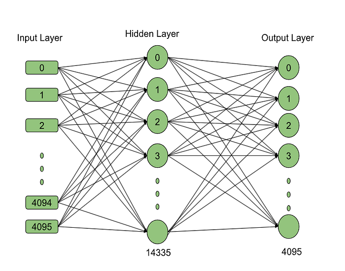
Image FFN: Numbers in the images are input and output dimensions from respective neurons.

I want to mention again, If you have a question why do we need FFN?

The attention Mechanism gives the relationship between words (Semantic, syntactic relationships, and how one words are related to others). But FFN learns to represent the words, It actually learns to write the sequence of the words from the attention information.

The FFN (Neural Network) is backed by the Universal approximation theorem (UAT). What does UAT say? It can approximate any ideal function in the real world. Same thing, the FFN learns to represent the language, it learns to write the words from the attention information.

The FFN takes the output from the attention layer, which has undergone RMS normalization, as its input. This input matrix has a shape of (9, 4096), where 9 represents the number of tokens or sequence length (i.e., the number of vectors), and 4096 is the model dimension.

Before we dive into the illustration of a feed-forward network, let’s take a closer look at the code of a FeedForward module from Mistral 7B.

class FeedForward(nn.Module):
 def __init__(self, args: ModelArgs):
 super().__init__()
 # Image 31 will represents pytorch linear layer operation.
 self.w1 = nn.Linear(args.dim, args.hidden_dim, bias=False)
 self.w2 = nn.Linear(args.hidden_dim, args.dim, bias=False)
 self.w3 = nn.Linear(args.dim, args.hidden_dim, bias=False)

 def forward(self, x) -> torch.Tensor:
 return self.w2(nn.functional.silu(self.w1(x)) * self.w3(x))

From this code, we can see that there are two hidden layer operations, not two hidden layers fully connected. Let’s break it down: the input matrix is fed into two hidden layers, self.w1, and self.w3, and then multiplied point-wise. The self.w1 hidden layer goes SiLU activation, But self.w3 does not.

This Operation is the SwiGLU Activation Function

SwiGLU(x) = SiLU (W_1.x).(W_3.x)

Why do they use two hidden layer operations(SwiGLU)? From my understanding, they have used another hidden layer operation to maintain the Magnitude of the vector, Because SiLU will reduce the Magnitude of all vectors, I will explain this in the SiLU Sub topic.

There are two hidden layers' weight matrices size is (14336,4096) as shown in images 20 and 20A.

The FFN hidden layer resulting matrix, with a shape of (9,14339), is then fed into the FFN output layer and multiplied by the output layer weight matrix, which has a shape of (4096,14336). This results in a feed-forward layer output with a size of (9,4096) as shown in image 21.

If you’re not familiar with how FFNs work, I recommend checking out my previous article on neural networks for a refresher.

Exploring Neural Networks: Fresh Perspective

Change your perspective about Neural Networks (MLP)!

medium.com

Image 22 provides a representation of the operations taking place within the Feed-Forward Network (FFN), which were previously explained in Images 20 and 21 ( x is the input vector, W1, W2, and W3 are weight matrix or parameters, Mistral didn’t use bias vector). In the vanilla Transformer model, the ReLU (Rectified Linear Unit) activation function was used. However, in Mistral, the SwiGLU activation function was used.

This Layer 1 output is then fed into the next layer or linear layer if there is no next layer. This helps us to predict the next token.

5. SiLU Activation Function ☺️

Though Mistral Architecture uses a SwiGLU activation function. we will Only Look into the SiLU activation function in this article.

When building neural networks, we use activation functions to add non-linearity to the model. Without non-linearity, the output would be directly proportional to the input, limiting the model to learning only linear relationships ( like lines or hyperplanes). By introducing the non-linear activation functions, the model can learn more complex patterns and curves in the data.

Sigmoid Linear Unit (SiLU)[6], aka the Swish activation function when the beta parameter is set to 1.

Sigmoid(x) = 1 / (1+(e^(-x)))

Swish Activation function = x * sigmoid(beta * x)

Sigmoid Linear Unit(SiLU) = x * sigmoid(x)

SwiGLU(x) = SiLU (W_1.x).(W_2.x)

Activation functions like the sigmoid have a potential drawback. They map input values (x) to a range between 0 and 1. This issue is related to the vanishing gradient problem. During backpropagation, if the gradients become too small, the model’s weights update very slowly and Causes problems in learning.

When these values(sigmoid output) are multiplied with the input vector (x) their magnitude will reduce unless the sigmoid output is 1. So that’s why Mistral uses another hidden layer in FFN and multiplies the output with a SiLU-activated hidden layer to maintain the magnitude of the vector that will be given to the next layer or linear layer on is called SwiGLU activation. SwiGLU and skip connections help maintain the magnitude of the vectors and prevent vanishing gradients and information loss.

6. KV Cache and KV Cache with Rolling Buffer Size 💕

Before we dive into KV cache or its variants, let’s take a step back and understand how inference works and the challenges that come with it.

6.1 Inference without KV Cache

I want to clarify One thing before the illustration: When we input the question “What is LLM?”, the model processes it all at once to start generating the answer. The key point is that the model does not predict the tokens of the question; it predicts the next token based on the entire input context (Auto-regressive). Let’s split the input question into 3 Tokens “What”, ”is”, and “LLM?”.

Note: For illustration purposes, I split into Only 3 tokens. Model split “?” as a separate token.

Imagine the process as illustrated in image 24

Note: [SOS] and [EOS] are virtual tokens, That help the model to indicate the start and end of the sequence. Not all LLM training and Inference use it.

Image 25 illustrates the inference from step 1 to step 3. Have a look at the size changes in Query, Key, Attention score, Value, and attention layer output.

From Image 24 you can see that the Initial Input question: [SOS] What is LLM?

Step 1:
Input: [SOS] What is LLM?
Predicted output: A

Step 2:
Input: [SOS] What is LLM? A
Predicted output: Large

Step 3:
Input: [SOS] What is LLM? A large
Predicted output: language

Step 4:

Input: [SOS] What is LLM? A large language
Predicted output: model

Step 5:

Input: [SOS] What is LLM? A large language model
Predicted output: is

And so on, The generation process continues until a stopping criterion is met. This could be a special end-of-sequence token [EOS], a maximum length limit, or some other predefined condition.

You might think everything is fine, but that’s not the case. During inference, when we need to predict the next token based on the context or previous token, we have to perform all the attention operations again from scratch. There are lots of unnecessary computations that were calculated previously. This is redundant and computationally expensive, creating a bottleneck. To overcome this, researchers introduced the KV cache method.

6.2 Inference with KV Cache

To achieve this, we maintain key and value vectors (the model needs access to all the previous tokens) and pass only the previously generated token to generate the next token. Images 26, 27, and 28 will give the complete picture of the KV cache during inference.

From Image 26 you can see that the Initial Input question: [SOS] What is LLM?

Step 1:
Input: [SOS] What is LLM?
Predicted output: A

Step 2:
Input: A
Predicted output: Large

Step 3:
Input: Large
Predicted output: language

Step 4:

Input: language
Predicted output: model

Step 5:

Input: model
Predicted output: is

And so on.

As I mentioned earlier, the next token is predicted based on the previous tokens. This is where the KV cache comes in. As the name suggests, the attention layer caches the key and value vectors to predict the next token. You can refer to Images 27 and 28 to get a better understanding of this concept.

Note: The Yellow color in the images 27 and 28 are new Query, key and value that was predicted previously

Note: Don’t look for sliding windows in Images 27 and 28. Till now we haven’t reached Mistal’s KV cache Variation 😃.

Let’s take a closer look at how this process works, as illustrated in Images 27 and 28. The key idea is that only the last predicted token is used in the next step. The cached Key and Value vectors retain their previous token vectors. This Predicted token is appended to the Key and Value vectors.

The last predicted token (Query only has the last predicted token)is multiplied by the cached Key vectors and then Cached Value vectors, resulting in an attention score matrix with a single row (1, 4096). This matrix contains attention information for all previous tokens. This vector is then fed into a Feed-Forward Network (FFN) and a Linear layer, which helps predict the next token.

This approach significantly reduces computation, as you can see by comparing Images 25 and 27. For example, Comparing Step 3 without the KV cache and with Cache, the KV cache method did very low and only needed computation.

In the Vanilla Transformer, self-attention is used to predict the next token, which involves calculating the attention for each token to all other tokens. However, with the KV cache method, we only need to create the last row of the attention matrix (That has all previous tokens' attention data), which allows us to predict the next token efficiently without losing accuracy.

6.3 KV Cache with Rolling Buffer Cache

Since we’re using sliding window attention, which has a window size of 4096 (Mistral architecture), we don’t need to store all previous tokens in the KV Cache. Instead, we can limit it to the latest tokens within the sliding window size. Therefore, we maintain the KV cache size to match the sliding window attention size.

Let’s take a closer look at how this works with a concrete example. Suppose our window size is 5. Steps 1–3 are the same as shown in Image 27. Steps 4 and 5 are shown in image 29. Since we’ve set the window size to 5, only vectors within this window are considered.

Even if we didn’t use a buffer size in the KV cache, all values outside the sliding window would become 0. In Mistral’s self-attention mechanism, tokens outside the sliding window are not attended to. Instead, the current token is attended to by previous tokens within the sliding window attention.

In other words, the current token is only influenced by the previous 4 tokens (since our window size is 5), and not by any tokens outside of this window. This is how Mistral’s self-attention mechanism efficiently focuses on the most relevant tokens when predicting the next token. We use the same property here in the KV cache as Buffer size as shown in Image 29.

Note: In Image 29, the Black colored area is removed to maintain the Window size of 5. Image 30 will give more understanding of what's happening in Key and value vectors.

Now, you might wonder why it’s called a Rolling Buffer. The answer lies in how the KV cache is updated. When a new token is generated, it is added to the end of the KV cache. If the KV cache is full, the next token is added to the front of the cache(the oldest token removed) and all remaining tokens shift forward to make place for the new token at the end. The added token goes to last in order. This is the essence of the “rolling” mechanism, where the buffer moves forward with each new token. Then this will fed into FFN and Linear Layer. You can understand from images 29 and 30.

6.4 Two more things in Inference are Pre-fill and chunking:

When generating a sequence from a large language model, we typically start with a prompt, such as “What is LLM?”. The model then generates tokens one by one, based on the previous tokens, thanks to its auto-regressive property. Since the prompt is already known, we can pre-fill the prompt token vectors in the KV cache. Using this KV cache, the next token is predicted, for example, “A”.

However, when the input prompt is very large, such as summarizing a book or a document, we need to break it down into smaller chunks, each of a fixed window size (chunk size = Window size). For each chunk, we compute the attention over both the cache and the chunk itself. For instance, the first vector of the second chunk needs to attend to the last vector of the first chunk, which is within the window size.

7. Linear Layer and Softmax in Mistral

Let’s walk through the first two steps of inference using our example, as shown in Image 27. The subsequent steps will follow the same method. As I mentioned earlier, the prompt is What is LLM?, which is split into three tokens: “What”, “is”, and “LLM?”. These tokens are then fed into the embedding model, followed by rotary positional embedding, sliding window attention, the feed-forward networks (FFNs), and finally, the linear layer.

Image 31: typical neural network (MLP, FFN, Linear Layer, and ANN) operation. x is the input vector, A is the weight matrix, and b is the bias vector.

# Output layer in Mistral. args.dim = model dimension, args.vocab_size = vocabulary size (32000)
self.output = nn.Linear(args.dim, args.vocab_size, bias=False)

As shown in Image 32, we can see the three vectors that have gone through the entire process, from the Embedding model to the Rotary positional encoding, and then through all the layer’s attention and FFN operations. The third vector, in particular, contains information about all the previous two tokens and the current token.

This vector is then multiplied by the linear layer weight matrix W_L, resulting in the linear layer output, as illustrated in Image 33. Finally, these linear layer outputs (logits) are fed into the softmax activation function, which gives us the highest probability of the next token (This is why LLM is often referred to as the probabilistic model). In our case, the predicted token is “A”. (“A” vocab index is 6097)

As we’re already familiar with the KV Cache and rolling buffer cache, the only predicted token “A” is fed back in as an input. It then goes through the entire process again, from the Embedding model to the Rotary positional encoding, and then through all the layer’s attention and FFN operations.

As shown in Image 34, the resulting vector now contains information about the original question and the predicted token “A”. This vector is then multiplied by the Linear layer weight matrix, producing a linear layer output of size (1,32000). These logits are then applied to the softmax activation function, which gives us the highest probability of the next token, which is “Large”, as shown in Image 35. (“Large”- vocab index is 3001)

Note: The weight matrix and bias vectors were updated during Backpropagation. The Mistral architecture didn’t used bias vector that you can understand from code. I tried my best to illustrate the workings of Mistral 7B. I hope you like it.

This same operation happens till the end of the answer. This is how the inference happens in Mistral 7B.

For fun, let’s calculate the total number of parameters in the model and compare it with the official size mentioned in the paper or website.

The Attention Layer Parameters Count can be calculated as :

No.of.layers x [(No.of.Query heads x query weight matrix size)+ k and V (No.of KV heads and KV head weight matrix)+ Linear projection in concatenated attention output]

= 32 x [(32 x 4096 x 128)+ 2(8 x 4096 x 128)+ (4096 x 4096)]
= 1,34,21,77,280

The Feed Forward Network Parameter Count can be calculated as:

No.of Layers x (2 x Hidden layer weight matrix + Output layer weight matrix )

= 32 x (2(14336 x 4096)+ (4096 x 14336))
= 5,63,71,44,576

The Linear Layer parameters count can be calculated as:
(4096 x 32000) = 13,10,72,000

The approximate total parameter count is:
1,34,21,77,280 + 5,63,71,44,576 + 13,10,72,000 = 7,11,03,93,856~ 7.11 Billion Parameters.

Officially, Mistral-7B-v0.1 has 7.24 Billion Parameters. We didn’t calculate the embedding network Parameters, Layer Normalization Parameters and we might have missed some additional layers or component parameters in the deep Mistral’s architecture.

We’ve explored many aspects of Mistral’s research paper. I recommend you develop a habit of proofreading and reading the original research papers and related materials to gain a deeper understanding and new perspectives.

If you found my article useful 👍, give it a👏! Feel free to follow for more insights.

Let’s also stay in touch on 🔗LinkedIn🌏❤️to keep the conversation going!

References:

[1]. Peter Shaw, Jakob Uszkoreit, Ashish Vaswani, Self Attention with Relative Position representation (2018)

[2]. Ashish Vaswani, Noam Shazeer, Niki Parmar, Attention is All You Need Research Paper (2017)

[3]. Jianlin Su, Yu Lu, Shengfeng Pan, Ahmed Murtadha, RoFormer: Enhanced Transformer with Rotary Position Embedding (2021)

[4]. Albert Q. Jiang, Alexandre Sablayrolles, Arthur Mensch, Mistral 7B (2023)

[5]. Umar Jamil, Mistral Architecture Explained, YouTube Video (2023)

[6]. Stefan Elfwing, Eiji Uchibe, Kenji Doya, Sigmoid-Weighted Linear Units for Neural Network Function Approximation in Reinforcement Learning (2017).

Join thousands of data leaders on the AI newsletter. Join over 80,000 subscribers and keep up to date with the latest developments in AI. From research to projects and ideas. If you are building an AI startup, an AI-related product, or a service, we invite you to consider becoming a sponsor.

Published via Towards AI