BERT: In-depth exploration of Architecture, Workflow, Code, and Mathematical Foundations

Author(s): JAIGANESAN

Originally published on Towards AI.

Delving into Embeddings, Masked Language Model Tasks, Attention Mechanisms, and Feed-Forward Networks: Not Just Another BERT Article — A Deep Dive Like Never Before🦸‍♂️

If you’ve been in the AI field for a while, you’ve likely come across BERT multiple times. Introduced in 2018, BERT has been a topic of interest for many, with lots of articles and YouTube videos attempting to break it down. However, this article takes a different approach.

Whether you’re looking to deepen your existing knowledge of BERT or are just starting your career in AI, this article aims to provide a comprehensive understanding of this concept.

Before We deep dive into BERT working Mechanism we need to understand what is the difference between BERT and Today’s LLM Models because Both use Transformer Architecture.

LLM is a Probabilistic and auto-regressive Model. Auto-Regressive in LLM Means, that LLM is trained to predict the next token ( Next token Prediction Task) based on the current context. LLM achieves this property by using a causal Mask in the Attention Layer, which helps tokens to attend only to previous tokens (Left Context), not future tokens in the sequence. This helps to predict the next tokens based on Current and previous tokens.

But BERT didn’t use a Causal Mask. So Each token attends other tokens in both directions (Left and right context). The objective of BERT is different. it was designed and trained on Tasks like Masked Language Model (MLM) and Next-sentence prediction (NSP) tasks. But By Fine-tuning BERT, It can be used on various tasks like classification and question-answering tasks.

Two types of BERT architecture were released in 2018, BERT Base, and BERT Large. The Bidirectional Transformer Architecture Model is often called the Encoder Model. Left Context transformer architecture (Causal mask applied) is often called a Decoder Model (LLM). Both BERT use WordPiece Tokenizer, which has a vocabulary size of 32000.

BERT Base Properties: 12 Encoder layers, 12 Attention Heads, Feed Forward Hidden Layer Size is 3072—total 110M Parameters. The embedding size is 768.

BERT Large Properties: 24 Encoder layers, 16 Attention Heads, Feed Forward Hidden Layer Size is 4096. Total 340M Parameters. The Embedding Size is 1024.

In this article, we will explore the BERT, based on the BERT Base architecture and Properties.

Image 1: BERT Base Architecture.

Let’s break down the BERT Base architecture, from word embeddings to linear and softmax layers. As discussed earlier, BERT was specifically designed for Masked Language Model (MLM) and Next Sentence Prediction (NSP) tasks. Here, we’ll only focus on the MLM task to understand the BERT Base architecture.

Let’s dive in!

Note: I haven’t delved into segment embedding from an architectural or theoretical perspective. The reason is that I’m planning to explore BERT based on the Masked Language Modeling (MLM) task, which doesn’t require segment embedding Segment embeddings help to segment the sequence in the Next sentence prediction task (NSP).

1. Masked Language Model (MLM)😷😂

Masked Language Model Task is nothing But a Cloze task. Train the Model to fill in the Blanks in the sentence. To illustrate this, let’s take a simple example. Suppose we have the sentence: “BERT Stands for Bidirectional Encoder Representation from Transformer”.

In this sentence, we remove the word “Encoder” and replace it with a special [Mask] virtual token indicating a blank space. The resulting sentence would be: “BERT Stands for Bidirectional [Mask] Representation from Transformer”. By giving this sentence to BERT, we train the Model to Predict the token “Encoder”. By Understanding the Input Model Predicts the Token.

Let’s Dive into the Components of BERT

2. Word Embeddings 🛤

I want to answer 3 questions on word Embeddings. What?, how?, why?. First, what are word embeddings? In simple terms, word embeddings are numerical representations of words or tokens in the form of vectors.

Next, how are sentences converted into Word Embeddings? Let’s take an example from the Masked Language Modeling (MLM) Topic. The sentence “BERT Stands for Bidirectional [Mask] Representation from Transformer” is broken down into tokens. Tokens are the smallest units of data, and can be words, special characters, or subwords.

After that, these tokens are converted into a vocabulary index, which is a one-hot representation vector that represents the tokens in the vocabulary. The vocabulary is simply a collection of unique tokens. Finally, these index representations are converted into vectors, which are multi-dimensional representations of words or tokens.

Note: The Numbers you see in the Images are for illustration purposes only.

As shown in Image 3, the sentence is converted into tokens, then vocabulary indices, and finally vectors. In this example, there are 8 tokens (although in real-world scenarios, the number of tokens may vary for this sentence). As a result, the input Embedding shape is (8,768), where 768 is the dimension of the BERT Base model.

So, why do we need word embeddings? The reason is that Models (Computers) can’t understand words; they only understand numbers. Therefore, words need to be converted into embeddings. These embeddings represent words in a multi-dimensional space.

As humans, we can easily understand the meaning of words and the relationships between them. For example, we know that “happy” and “joy” have similar meanings, while “happy” and “sad” have opposite meanings. But how do models understand these relationships? The answer lies in vectors. In the multi-dimensional space, words with similar meanings are located close together, while words with dissimilar meanings are far apart from each other.

But, Wait a minute, How are similar embeddings near each other in Multi-dimensional space?

Well, the answer is by training the Model. Initially, embeddings are randomly initialized. As the model continues to train, Tokens that are similar in meaning start to cluster together in the multidimensional space.

import torch.nn as nn
class TokenEmbedding(nn.Embedding):
 def __init__(self, vocab_size, embed_size=768):
 super().__init__(vocab_size, embed_size, padding_idx=0) 
# Vocab Size is 32000 in BERT and Embed_Size is 768.
# nn.Embeddings Create Embeddings with the size of (32000,768)

2. Position Embeddings

Position embeddings play a crucial role in providing the model with information about the position of each token in the sequence. But why do we need position embeddings in the first place?

The answer is that without them, the model wouldn’t be able to understand the position of a token in the sequence. This means that even if the same word appears in different positions, the model would treat it as the same. For example, in the sentence “BERT is a great model” and “Is BERT a great model?”, the word “BERT” appears in different positions, but without position embeddings, the model would fail to recognize this difference.

In BERT, positional embeddings are created using the same method as word Embeddings, Not the Sinusoidal function that is mentioned in the “attention is all you need” paper. In BERT the Maximum position Embedding is limited to 512. This means only 512 tokens get their positional information. It’s also one of the reasons that BERT can’t be used in a wide range of tasks. And This Positional Information is Learnable. It gets updated during Backpropagation. Positional Embeddings learns 512 positional information during training. These position Embeddings are absolute, and represent only tokens' position.

# Official BERT (Github) Code is in Tensorflow. I have changed this into Pytorch version. 
# Checkout References [3,4] for more.

seq_length = 128 # Example sequence length
max_position_embeddings = 512
embed_size = 768

# Embeddings are created and trained for Max sequence length (512)
full_position_embeddings = nn.Embedding(max_position_embeddings, embed_size) 

# The Position Embeddings are sliced into input sequence length
# if the sequence length is small compare to maximum position
position_ids = torch.arange(seq_length, dtype=torch.long)
position_embeddings = full_position_embeddings(position_ids)

# positional Embeddings are added into 
input_embeddings = word_embeddings + position_embeddings

3. Input Embeddings

The Word Embeddings are added (point-wise addition) with position Embeddings. These Embeddings are given to the Encoder Layer in the BERT architecture. These input Embeddings have both Word and its position information in the sequence.

4. Self Attention

Now that we’ve explored word embeddings and position embeddings in BERT, it’s time to delve into the self-attention mechanism. To fully understand multi-head attention, we need to understand self-attention clearly.

Self-attention consists of three key components: Query, Key, and Value. Interestingly, these three components are identical and are either the input embeddings or derived from the output of the previous Encoder layer.

What is self-attention? In simple terms, self-attention is a Method where the input sequence is compared against itself to determine the importance of other words or tokens with respect to the current word. This allows the model to capture dependencies and relationships between words within the sequence, regardless of their positions. As a result, the model can understand the semantic and syntactic relationships between words in the input sequence.

Image 6 gives a mathematical equation of self-attention. The Query and the transposed Key are multiplied ( Vector_1. Vector_2), and then the result is divided by the square root of the model’s dimension, which is the square root of 768 in our case.

Next, a softmax function is applied row-wise to the resulting matrix. Finally, the output is multiplied by the Value vector matrix, which gives the self-attention output.

As shown in image 7 the Key and Query vector matrix are multiplied and divided by the root of (768). The resulting matrix will be a size of (8,8). It has the Attention logits of Each token with other tokens in the sequence.

The resulting matrix is then fed into a softmax function, which outputs a set of probabilities or attention scores. These attention scores show how each token has dependencies or semantic and syntactic relationships with other tokens in the sequence. In other words, they show how important each token is to every other token in the sequence.

Then the attention score matrix (8,8) is multiplied by the Value vectors Matrix resulting in the attention output (8,768). In this attention output, each token has information on other tokens. It combines the information about how the words are related to each other based on attention score. This information is then fed into a feedforward neural network.

class Attention(nn.Module):
 def forward(self, query, key, value, mask=None, dropout=None):
 scores = torch.matmul(query, key.transpose(-2, -1)) \
 / math.sqrt(query.size(-1))

 if mask is not None:
 scores = scores.masked_fill(mask == 0, -1e9)

 p_attn = F.softmax(scores, dim=-1) # Attention Score
 return torch.matmul(p_attn, value) # Attention Layer output

5. Multi-Head Attention

As we have seen, self-attention captures the relationship between words, then Why do we need Multi-Head attention 🤔? Self-attention captures the relationship between words in one Perspective (It may capture the order of the sequence, grammatical structure, Context, or dependencies between words). But Multi-Head attention captures the relationship between words in different perspectives with the help of weights (Parameters). We do self-attention with model dimensional, But Multi-Head attention with head’s dimension.

The Query(Q), Key(K), and Value(V) are Identical. It is Input Embeddings or Comes from the Previous Enocder Layer.

We know BERT Base’s Model dimension is 768 and The multi-head attention layer has 12 heads. To calculate the dimension of each head, we simply divide 768 by 12, which gives us 64.

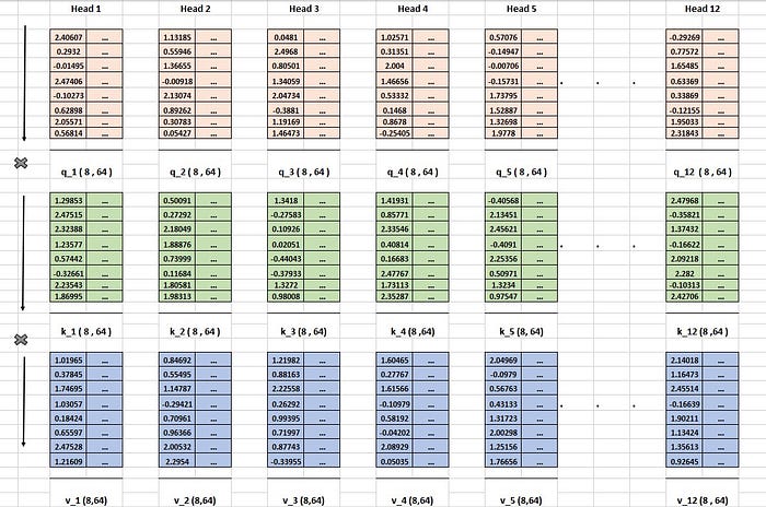
For each of these 12 heads, we need three components: query, key, and value vector matrices. This means we’ll have 12 separate attention mechanisms in the multi-head attention layer. Each attention operation captures different perspectives of the input sequence.

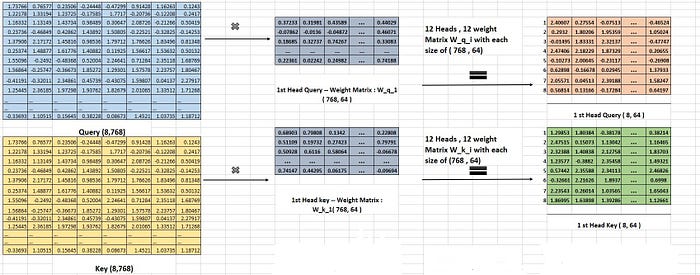
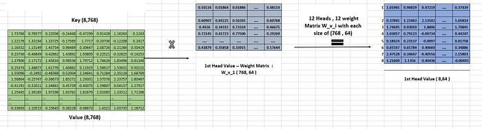
But how are these query, key, and value matrices created? As shown in Image 10 and illustrated in Images 12 and 13, To create the query vector matrices, we multiply it with 12 query weight matrices (In Practice, this operation is a little bit different, I explained in the Code section), each with a size of (768,64). This gives us 12 query vector matrices, one for each head, with a size of (8,64). Here, 64 represents the dimension of the head, and 8 represents the number of tokens in our example. The same process is repeated to create the key and value vector matrices for all heads.

Image 11 gives the linear layer operation in pytorch. As I’ve emphasized in my previous articles, when it comes to linear layers or neural networks, it’s essential to think in terms of matrices and vectors rather than neurons. In Image 11, we can see that the input vector x (embeddings, vectors) is multiplied by the transposed weight matrix A. The weight matrix A has a size of (output feature size, input feature size). Additionally, the bias vector b is broadcasted into each row of the resulting matrix.

Within each head, the same self-attention operation takes place, using the respective query, key, and value vector matrices. Let’s take the first head as an example. Here, the query_1 matrix (with a size of 8,64) is multiplied by the transposed key_1 matrix (also with a size of 8,64), resulting in an 8×8 matrix.

Next, this resulting matrix is divided by the square root of the key’s dimension, which is 8 (since the key’s dimension is 64). Finally, the result is multiplied by the value vector matrix, producing the attention output for head 1, with a size of 8,64.

This same operation is repeated for all 12 heads, generating 12 attention head outputs, each with a size of 8,64. This MHA operation is illustrated in images 14 and 15.

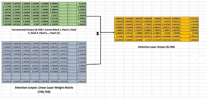
Ultimately, these outputs from all the heads are concatenated, resulting in a single output with a size of 8,768. The resulting Concatenated output is linearly projected with a weight matrix size of (768,768), resulting in Multi-Head attention Layer Output with a size of (8,768) as shown in Image 16.

Up until now, we’ve explored the mathematical representations and illustrations of the Multi-Head Attention mechanism. Now, let’s dive into the code level and see how it’s implemented in PyTorch. The following code snippet will give you a better understanding of how MHA works in practice.

class MultiHeadedAttention(nn.Module):
 def __init__(self, h, d_model, dropout=0.1):
 super().__init__()
 assert d_model % h == 0 # make sure remainder is 0, otherwise it will throug an error
 self.d_k = d_model // h # Head's dimension
 self.h = h # No.of Heads

 self.linear_layers = nn.ModuleList([nn.Linear(d_model, d_model) for _ in range(3)])
 self.output_linear = nn.Linear(d_model, d_model) #Output Linear layer (768,768)
 self.attention = Attention() #Attention funtion

 def forward(self, query, key, value, mask=None):
 batch_size = query.size(0) # Input sequence length
"""
** As we've seen earlier, the theory suggests that 12 separate weight matrices, 
each with a size of (sequence length, head's dimension), are used to create 
the 12 query matrices for Multi-Head Attention. This is exactly how we seen 
illustration. 
However, in practice, things work a bit differently. Instead of 
using 12 separate weight matrices, a single linear layer weight matrix with a 
size of (8,768) is used to project the query. This projected query is then 
sliced into 12 separate queries, each with the head's dimension. The same 
approach is applied to the key and value matrices as well.

In Both Practices the Output queries and the number of parameters are same. But 
This approach is efficient.
"""


 # 1) Do all the linear projections in batch from d_model => h x d_k
 query, key, value = [l(x).view(batch_size, -1, self.h, self.d_k).transpose(1, 2)
 for l, x in zip(self.linear_layers, (query, key, value))]

 # 2) Apply attention on all the projected vectors
 x, attn = self.attention(query, key, value, mask=mask, dropout=self.dropout)

 # 3) "Concat" using a view 
 x = x.transpose(1, 2).contiguous().view(batch_size, -1, self.h * self.d_k)

 return self.output_linear(x) # Apply a final linear(Attention Layer output)

6. Feed Forward Network

In its simplest form, a feed-forward network is a type of neural network that consists of three main layers: an input layer, a hidden layer, and an output layer. The number of input units in the input layer and the number of neurons in the output layer is the size of the model’s dimension (768). Interestingly, in the case of BERT, the hidden layer is typically four times (3072) the size of the model’s dimensions.

Why do we need FFN (Feed Forward Network)? The attention Mechanism helps to get the information about the sequence. The attention layer helps capture the semantic and syntactic relationships between words in the sequence and contextual understanding of the sequence. But Feed Forward Network Learns these representations, sequence from attention output. It approximates the Language humans use to communicate. By Learning the sequence it can predict the tokens.

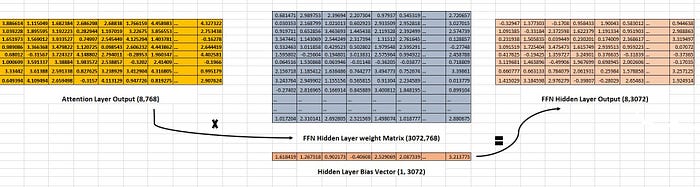
The output from the Multi-Head attention layer, which has a size of (8,768), is fed into the input layer of the Feed-Forward Network (FFN). Think of the input layer as a bridge that simply passes on the information without performing any operations.

The input (8,768) is then multiplied by the FFN hidden layer weight matrix with a size of (3072,768), resulting in a matrix size of (8,3072). Next, a bias vector (1,3072) is added to each row of the resulting matrix, a process known as broadcasting. This process gives hidden layer output.

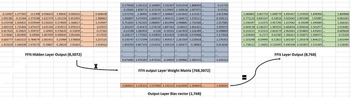
The output from the hidden layer (8,3072) is then multiplied by the FFN output layer weight matrix with a size of (768,3072), resulting in a vector-matrix size of (8,768). Finally, an output layer bias vector (1,768) is added to each row, completing the FFN layer output. This output is then passed on to the next encoder layer or a linear layer at the end. The Bias vector changes the vectors little bit, It actually helps to generalize the Model.

In BERT, the GELU (Gaussian Error Linear Unit) activation Function is used. The GELU activation function combines properties of both ReLU and Gaussian Noise to provide a smoother and more continuous approximation. It can approximate as you have seen in image 20 or GELU ~ x. sigmoid (1.702 x).

Let’s Understand the FFN Code

class PositionwiseFeedForward(nn.Module):
# d_ff is dimension of feed forward which is 3072
# d_model is model dimension (768)
 def __init__(self, d_model, d_ff, dropout=0.1):
 super(PositionwiseFeedForward, self).__init__()
 self.w_1 = nn.Linear(d_model, d_ff) 
 self.w_2 = nn.Linear(d_ff, d_model)
 self.activation = GELU()

 def forward(self, x):
 return self.w_2((self.activation(self.w_1(x))))

7. Linear Layer and Softmax in MLM

After all the Encoder layers (12), the final Matrix (8,768) is fed into the linear layer to predict the exact token for the Masked Language Model (MLM) Tasks.

The vector matrix (8,768) is then fed into a linear layer, where it’s multiplied by the linear layer weight matrix (32000,768). This results in a new matrix with a size of (8,32000), where 32000 represents the total number of words in the vocabulary. This resulting matrix is called the logits matrix.

Next, the softmax function is applied to the logits matrix, which assigns a probability score for logits to each row. The index with the highest probability score is selected as the output token.

The loss works similarly. The target matrix (8,32000) is sparse, meaning it has mostly zero values, except for the target index which is set to one. This helps to calculate the loss, update the gradients, and train the BERT model for the task.

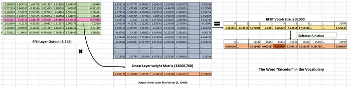
When the masked virtual token vector (in this case, the 5th token) is passed through the linear layer, it produces a logit matrix with a size of (1,32000). This matrix is then fed into the softmax function, which generates probability scores across all 32000 possible tokens.

The token with the highest probability is selected as the output token. In our example, The correct output is the token “Encoder”, which has an index of 15434 in the vocabulary. The probability at an index of 15434 should be high in order to give the output as “Encoder”. This means that the model is confident that the correct output is “Encoder” as shown in image 22.

class MaskedLanguageModel(nn.Module):

# hidden --> Model's dimension (768)
# Vocab_size --> Vocabulary size (32000)
 def __init__(self, hidden, vocab_size):
 super().__init__()
 self.linear = nn.Linear(hidden, vocab_size)
 self.softmax = nn.LogSoftmax(dim=-1)

 def forward(self, x):
 return self.softmax(self.linear(x))

Important note: It’s important to remember that the weight matrices, bias vectors, position embeddings, and word embeddings are all learnable. This means that they get updated during the backpropagation process while the model is being trained.

And that’s a wrap! We’ve reached the end of this article. I must admit, there are some topics we didn’t cover, such as segment embeddings, next-sentence prediction tasks, and fine-tuning BERT for specific tasks. However, I believe we’ve covered the most essential topics to give you a solid understanding of the BERT architecture.

By grasping the architecture, you’ll be able to modify the loss function and BERT architecture to suit your specific use case. This knowledge will empower you to tailor BERT to your needs and unlock its full potential.

Thanks for reading this article 🤩. If you found my article useful 👍, give Clapssss👏😉 ! Feel free to follow for more insights.

Let’s stay connected and explore the exciting world of AI together!

Join me on LinkedIn: linkedin.com/in/jaiganesan-n/ 🌍❤️

If you’re really interested in Advance LLM, NLP, and Gen AI, and you have some spare time, I invite you to explore my articles on these topics.

Exploring LLM: A Collection of My Articles❤️

Dive into the intricate world of large language models with in-depth articles on their architectures, MoE, and RAG…

medium.com

References:

[1] Ashish Vaswani, Noam Shazeer, Niki Parmar, Jakob Uszkoreit, Llion Jones, Attention is all you Need (2017). Research Paper (Arxiv).

[2] Jacob Devlin, Ming-Wei Chang, Kenton Lee, Kristina Toutanova, BERT Research Paper 2018.

[3] BERT- Pytorch Implementation, GitHub Repo (2018)

[4] BERT- Tensorflow Implementation, Official Github repository given in BERT Research Paper, 2018

[5] Gaussian Error Linear Unit (GELU)

Join thousands of data leaders on the AI newsletter. Join over 80,000 subscribers and keep up to date with the latest developments in AI. From research to projects and ideas. If you are building an AI startup, an AI-related product, or a service, we invite you to consider becoming a sponsor.

Published via Towards AI